2. Beijing Institute of Long March Vehicle, Beijing 100076, China ;
3. Research Center of Satellite Technology, Harbin Institute of Technology,Harbin 150001, China
In recent years,it has witnessed a tremendous research interest in the spacecraft missions that consist of multiple space vehicles,such as spacecraft formation flying,autonomous rendezvous and proximity operations[1-3]. A successful implementation of these multiple-spacecraft missions is highly dependent on the ability to determine the relative motion between the spacecraft. Typically,to estimate the relative spacecraft motion,it requires both high-fidelity dynamical models and specialized measurement methods.
The relative motion between two spacecraft is a six-degree-of-freedom (6-DOF) motion,which is composed of relative rotational motion,relative translational motion and the coupling thereof[4]. A growing interest has been paid for the modeling of 6-DOF spacecraft relative motion in recent years. For example,Pan and Kapila[5] addressed the coupled translational and rotational dynamics for the leader-follower spacecraft formation; Kristiansen[6] derived the Lagrange-like 6-DOF model by combining the relative translational dynamics and the rotational one. It is worth pointing out that the translational parts in the aforementioned models only account for the relative position between the centers of the mass (c.m.) of two spacecraft,and the rotation-translation coupling in this case is just induced by external torques. However,in general missions,the relative translational dynamics of arbitrary points on the spacecraft may be concerned. Whenever one of these points does not coincide with the spacecraft’s c.m,a kinematic coupling,which is essentially a projection of the rotational motion about the c.m. onto the relative translational configuration space,is obtained[4]. It is this kinematic coupling that the current paper is concerned with. As shown in the previous work,dual quaternion has been an effective tool for motion description and dynamics modeling[7-13].Among these works,Wang[13] was the first to use dual quaternion for spacecraft motion modeling.To go further step,this paper employs dual quaternion to model the relative motion between arbitrary points of spacecraft,and derives the kinematically-coupled relative dynamics.
Estimating the relative motion also involves the problem of sensing the relative information between spacecraft. In the past years,the single vision-based method has been used widely for the pose estimation problem [14-15]. Primary researches have focused on using two-dimensional/three-dimensional (2D/3D) point correspondences[16-19]. Among these literatures,Kim [18] and Xing [19] employed the line-of-sight (LOS) measurements and Extended Kalman Filter (EKF) to estimate the relative position and attitude for spacecraft. However,the point-based methods are often limited to the difficulty of point matching and high sensitivity to noise. In view of these issues,several researchers have investigated the pose estimation problem based on higher-level geometric features such as lines and curves. For instance,using a set of 2D/3D line correspondences,the direct solutions[20-21],and the iterative method [22-23] have been proposed to estimate the external camera parameters. From a pair of conics in both 2D and 3D,Song[24] introduced an iterative technique for the pose estimation problem. However,to the best knowledge of the authors,these methods have been seldom used for spacecraft relative motion estimation problem. In addition,nearly all the existing solutions concentrate on one specific type of correspondences,that is,they either use points or lines or conics but not a combination of features. In order to improve the robustness and accuracy for estimating the relative motion,this paper describes the feature points,lines and circles in dual number algebra,and establishes an integrated observation model based on multiple geometric features.
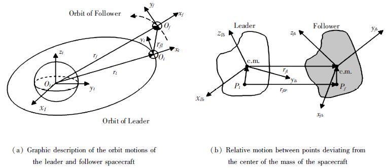
2 Kinematic-Coupled Dynamics Model Using Dual NumberThroughout the development of the dynamics model,some standard reference frames are to be used (see Fig. 1): ΨI,the standard Earth-centered,inertial,Cartesian right-hand reference frame; Ψl,a local-vertical,local-horizontal reference frame fixed to the c.m. of leader spacecraft,with its xl axis directing from the spacecraft radially outward,zl axis normal to the leader orbital plane,and yl axis set up by the right-hand rule; Ψlb (resp. Ψfb),the body-fixed reference frame of the leader spacecraft (resp. the follower spacecraft),with its origin in the center of mass of the spacecraft,and axes pointing along the principal axes of inertia. In the following discussion,it is assumed that the leader orbital frame Ψl is controlled aligned with the body-fixed frameΨlb.
|
Figure 1 Defination of reference frames |
As shown in Fig. 1(b),there exists an arbitrary feature point Pl located on the leader spacecraft. Let pll be the position vector directed from the point Pl to the c.m. of the leader spacecraft. By translating the coordinate system Ψlb along the opposite direction of pll ,one can obtain a new coordinate system ΨlP with its origin being the point Pl,and axes parallel to those of Ψlb. In the same way,a new coordinate system ΨfP for the follower spacectaft is also derived.
In the remainder of this paper,the following notations are employed:
By definingthe operations
| $\left\{ \begin{align} & \hat{\omega }_{lP}^{lP}=\hat{\omega }_{lP}^{l}={{{\hat{P}}}_{l}}\hat{\omega }_{l}^{l} \\ & \hat{\omega }_{fP}^{fP}=\hat{\omega }_{fP}^{f}={{{\hat{P}}}_{f}}\hat{\omega }_{f}^{f} \\ \end{align} \right.$ | (1) |
where
| $2{{\dot{\hat{q}}}_{fl,P}}={{\hat{q}}_{fl,P}}\cdot {{\hat{\omega }}_{fPfl,P}}$ | (2) |
where
In terms of Eq. (1),
| $\hat{\omega }_{fl,P}^{fP}={{\hat{P}}_{f}}\hat{\omega }_{f}^{f}-\hat{q}_{fl,P}^{*}\cdot \left( {{{\hat{P}}}_{l}}\hat{\omega }_{l}^{l} \right)\cdot {{\hat{q}}_{fl,P}}$ | (3) |
where
| $\begin{align} & \dot{\hat{\omega }}_{fl,P}^{fP}={{{\hat{P}}}_{f}}\dot{\hat{\omega }}_{f}^{f}-\hat{q}_{fl,P}^{*}\cdot \left( {{{\hat{P}}}_{l}}\dot{\hat{\omega }}_{l}^{l} \right)\cdot {{{\hat{q}}}_{fl,P}}- \\ & \hat{q}_{fl,P}^{*}\cdot \left( {{{\hat{P}}}_{l}}\hat{\omega }_{l}^{l} \right)\cdot \hat{q}_{fl,P}^{\cdot }- \\ & \dot{\hat{q}}_{fl,P}^{*}\cdot \left( {{{\hat{P}}}_{l}}\hat{\omega }_{l}^{l} \right)\cdot {{{\hat{q}}}_{fl,P}} \\ & ={{{\hat{P}}}_{f}}\dot{\hat{\omega }}_{f}^{f}-\hat{q}_{fl,P}^{*}\cdot \left( {{{\hat{P}}}_{l}}\dot{\hat{\omega }}_{l}^{l} \right)\cdot {{{\hat{q}}}_{fl,P}}- \\ & \hat{q}_{fl,P}^{*}\cdot \left( {{{\hat{P}}}_{l}}\hat{\omega }_{\text{l}}^{\text{l}} \right)\cdot \frac{1}{2}{{{\hat{q}}}_{fl,P}}\cdot \hat{\omega }_{fl,P}^{f}+ \\ & \frac{1}{2}\hat{\omega }_{fl,P}^{\text{f}}\cdot \hat{q}_{fl,P}^{*}\cdot \left( {{{\hat{P}}}_{l}}\hat{\omega }_{l}^{l} \right)\cdot {{{\hat{q}}}_{fl,P}} \\ & ={{{\hat{P}}}_{f}}\left( -\hat{M}_{f}^{-1}\left( \hat{\omega }_{f}^{f}\times {{{\hat{M}}}_{f}}\hat{\omega }_{f}^{f} \right)+\hat{M}_{f}^{-1}\hat{F}_{f}^{f} \right)- \\ & \hat{q}_{fl,P}^{*}\cdot \left( {{{\hat{P}}}_{l}}\dot{\hat{\omega }}_{l}^{l} \right)\cdot {{{\hat{q}}}_{fl,P}}+\hat{\omega }_{fl,P}^{f}\times \\ & \left( \hat{q}_{fl,P}^{*}\cdot \left( {{{\hat{P}}}_{l}}\hat{\omega }_{l}^{l} \right)\cdot {{{\hat{q}}}_{fl,P}} \right) \\ \end{align}$ |
where the dual inertia matrix of the follower spacecraft is given by
Before developing the observation models in this section,two reference frames are defined. The camera reference frame Ψc,a 3D Cartesian right-hand coordinate system with its origin is located at the lens center of the camera,xc axis along the horizontal direction of the image,yc axis along the vertical direction of the image,and zc axis parallel to the optical axis of the camera. The image reference frame Ψi,a 2D coordinate system,contained in the image plane,and is parallel to the xc and yc axes of Ψc. Without loss of generality,it is assumed that Ψc is aligned with ΨfP which is defined in the previous section.
3.1 Observation Model Based on Feature PointsIn this subsection,the pinhole lens model is used as the perspective projection model,and the process of a 3-D point to its 2-D projection is briefly summarized as follows.
Let D be a 3D point fixed on the leader spacecraft. The first step is to transform the point D to the camera reference frame. In the dual quaternion algebra,this transformation can be expressed as
| ${{\hat{D}}^{fP}}=\hat{q}_{fl,P\varepsilon }^{*}{{\hat{D}}^{lP}}{{\hat{q}}_{fl,P}}$ |
where
Next step is to project the transformed points onto the image plane. The result is the x and y coordinates of the projected points. Given the camera coordinates
| ${{x}_{id}}=\lambda \frac{{{d}_{fpx}}}{{{d}_{fpz}}},{{y}_{id}}=\lambda \frac{{{d}_{fpy}}}{{{d}_{fpz}}}$ | (4) |
where λ is the focal length of the camera.
3.2 Observation Model Based on Feature LinesIn this section,the given model features from the leader spacecraft are lines. The projection of a 3D line onto the 2D image is shown in Fig. 2. In the dual quaternion algebra,the expression of the feature line L relative to ΨlP is represented by

|
Figure 2 Observation model based on feature Lines |
| ${{\hat{L}}^{lP}}={{l}^{lP}}+\varepsilon {{m}^{lP}}$ |
where llP denotes the unit direction vector and mlP is the moment with respect to the origin of ΨlP. Using dual quaternion,one can calculate the expression of
| ${{\hat{L}}^{fP}}={{l}^{fP}}+\varepsilon {{m}^{fP}}=\hat{q}_{fl,p}^{*}\cdot {{\hat{L}}^{lP}}\cdot {{\hat{q}}_{fl,p}}$ | (5) |
Perspective projection is then applied to the transformed lines. In terms of projection geometry,an equation of the projected line is obtained:
| ${{m}_{x}}{{x}_{i}}+{{m}_{y}}{{y}_{i}}={{m}_{z}}\lambda $ | (6) |
where xi and yi are the image plane coordinates. From Eq. (9),one can calculate the direction vector of the image line by
| ${{l}_{i}}={{\left[ \begin{matrix} {{l}_{ix}} & {{l}_{iy}} & {{l}_{iz}} \\ \end{matrix} \right]}^{\text{T}}}={{\left[ \begin{matrix} \frac{-{{m}_{y}}}{\sqrt{m_{x}^{2}+m_{y}^{2}}} & \frac{{{m}_{x}}}{\sqrt{m_{x}^{2}+m_{y}^{2}}} & 0 \\ \end{matrix} \right]}^{\text{T}}}$ | (7) |
Since the momentum of the image line mi defines the same plane as m,one may have
| ${{m}_{i}}={{\left[ \begin{matrix} {{m}_{ix}} & {{m}_{iy}} & {{m}_{iz}} \\ \end{matrix} \right]}^{\text{T}}}={{d}_{pc}}\frac{m}{\left\| m \right\|}=\frac{\lambda }{\sqrt{m_{x}^{2}+m_{y}^{2}}}m$ |
where dpc is the distance from the image line to the perspective center.
A format is needed to compare these transformed lines with lines measured from the acquired images. In Fig. 2(b),the line point[23],which is defined as the intersection of the line feature with a line passing through the image origin that is perpendicular to the line feature,is employed. From the image line,the coordinates of the line point are calculated as
| ${{x}_{il}}={{l}_{iy}}{{m}_{iz}},{{y}_{il}}=-{{l}_{ix}}{{m}_{iz}}$ | (8) |
In terms of Eqs. (7) and (8),the line point can be also derived from the 3D transformed line by the equation:
| ${{x}_{il}}=\lambda \frac{{{m}_{x}}{{m}_{z}}}{m_{x}^{2}+m_{y}^{2}},{{y}_{il}}=\lambda \frac{{{m}_{y}}{{m}_{z}}}{m_{x}^{2}+m_{y}^{2}}$ | (9) |
Therefore,the relations between the line point from the acquired image and the 3D line on the leader spacecraft are established by Eqs. (5) and (9),and these equations can be used as the observation model for the estimation problem.
3.3 Observation Model Based on Feature CirclesBesides the point and line features,circle features are also common tobe found on a spacecraft. However,in the dual quaternion algebra,circles cannot be represented and transformed directly like the way of the points and lines. For the aim of dealing with all the three types of features in a unified algebra,this section proposes an operation definition for circles. With this definition,the equations which related the 3D circles and 2D conics are formalized accordingly.
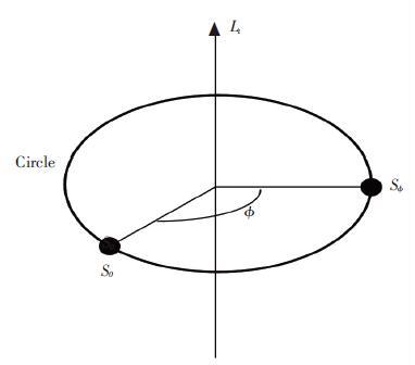
As shown in Fig. 3,a circle can be regarded as a twist Lt modeling a general rotation and a starting point S0 on the circle. According to the definition of screw motion,this twist transformation can be understood as a screw motion with the screw pitch being zero.Given the generating twist parameters,the twist transformation corresponds to the dual quaternion:
|
Figure 3 The operational definition of circles |
| ${{\hat{q}}_{\phi }}=\left[ \cos \frac{\phi }{2},{{{\hat{L}}}_{t}}\sin \frac{\phi }{2} \right]$ |
where
| $\hat{S}_{\phi }^{lP}={{\hat{q}}_{\phi }}\hat{S}_{0}^{lP}\hat{q}_{\phi ,\varepsilon }^{*}$ | (10) |
where
| $\hat{S}_{\phi }^{fP}=1+\varepsilon S_{\phi }^{fP}=q_{fl,P\varepsilon }^{*}\hat{S}_{\phi }^{lP}{{\hat{q}}_{fl,P}}$ |
In terms of Eq. (4),the image coordinates of the point Sφ are calculated by
| ${{x}_{is}}=\lambda \frac{{{s}_{\phi fPx}}}{{{S}_{\phi fPz}}},{{y}_{is}}=\lambda \frac{{{s}_{\phi fPy}}}{{{S}_{\phi fPz}}}$ | (11) |
where sφfPx,sφfPy and sφfPz are the components of the sφfP.
Taking the image coordinatesxis,yis as the measurement variables,the observation model based on the circle features is now set up with the above equations.It should be noted that
The state vector of the system is selected as
| $X={{\left[ \begin{matrix} {{{\hat{q}}}_{fl,P}} & \hat{\omega }_{fl,P}^{fP} & \Phi \\ \end{matrix} \right]}^{\text{T}}}$ |
where Φ=[φ1…φ3n] are the unknown parameters of the observed n feature circles. Based on the kinematics and dynamics proposed in Section 2,one may have the following continuous-time process model:
| $\dot{X}\left( t \right)=f\left( X\left( t \right),t \right)+w\left( t \right)$ |
where f(X(t),t) is a non-linear function given by
| $\begin{align} & f\left( X\left( t \right),t \right)={{\left[ \begin{matrix} {{{\dot{\hat{q}}}}_{fl,P}} & \dot{\hat{\omega }}_{fl,P}^{fP} & {\dot{\Phi }} \\ \end{matrix} \right]}^{\text{T}}}= \\ & \left[ \begin{matrix} \frac{1}{2}{{{\hat{q}}}_{fl,P}}\cdot \hat{\omega }_{fl,P}^{fP} \\ \begin{matrix} {{{\hat{P}}}_{f}}\left( -\hat{M}_{f}^{-1}\left( \hat{\omega }_{f}^{f}\times {{{\hat{M}}}_{f}}\hat{\omega }_{f}^{f} \right)+\hat{M}_{f}^{-1}\hat{F}_{f}^{f} \right)- \\ \hat{q}_{fl,P}^{*}\cdot \left( {{{\hat{P}}}_{l}}\dot{\hat{\omega }}_{l}^{l} \right)\cdot {{{\hat{q}}}_{fl,P}}+\hat{\omega }_{fl,P}^{fP}\times \left( \hat{q}_{fl,P}^{*}\cdot \left( {{{\hat{P}}}_{l}}\hat{\omega }_{l}^{l} \right)\cdot {{{\hat{q}}}_{fl,P}} \right) \\ \end{matrix} \\ {{0}_{3n\times 1}} \\ \end{matrix} \right] \\ \end{align}$ |
where w(t) is a white Gaussian process noise with power spectral density matrix Q.
Linearizing and discretizing of the process model yields
| ${{X}_{k}}={{F}_{k,k-1}}{{X}_{k-1}}+{{W}_{k-1}}$ |
where Fk,k-1=I+Ck-1T with T being the sample time,and
| ${{\left. {{C}_{k-1}}=\frac{\partial \text{f}}{\partial {{X}^{\text{T}}}} \right|}_{X={{X}_{k-1}}}}=\left[ \begin{matrix} \frac{\partial {{{\dot{\hat{q}}}}_{fl,P}}}{\partial {{{\hat{q}}}^{\text{T}}}_{fl,P}} & \frac{\partial {{{\dot{\hat{q}}}}_{fl,P}}}{\partial \hat{\omega }_{fl,P}^{fPT}} & {{0}_{8\times 3n}} \\ \frac{\partial {{{\dot{\hat{\omega }}}}_{fl,P}}}{\partial {{{\hat{q}}}^{\text{T}}}_{fl,P}} & \frac{\partial {{{\dot{\hat{\omega }}}}_{fl,P}}}{\partial {{{\hat{\omega }}}^{fPT}}_{fl,P}} & {{0}_{6\times 3n}} \\ {{0}_{3n\times 8}} & {{0}_{3n\times 6}} & {{0}_{3n\times 3n}} \\ \end{matrix} \right]$ |
with the expressions given as follows:
| $\begin{align} & \frac{\partial {{{\dot{\hat{q}}}}_{fl,P}}}{\partial {{{\hat{q}}}^{\text{T}}}_{fl,P}}=\frac{1}{2}\left[ \hat{\omega }_{fl,P}^{fP-} \right],\frac{\partial {{{\dot{\hat{q}}}}_{fl,P}}}{\partial \hat{\omega }_{fl,P}^{fPT}}=\frac{1}{2}\left[ \hat{q}_{fl,P}^{+} \right] \\ & \frac{\partial {{{\dot{\hat{\omega }}}}_{fl,P}}}{\partial {{{\hat{q}}}^{\text{T}}}_{fl,P}}=-\left( {{\left[ \hat{q}_{fl,P}^{+} \right]}^{\text{T}}}\left[ {{\left( {{{\hat{P}}}_{l}}\hat{\omega }_{l}^{l} \right)}^{+}} \right]+ \right. \\ & \left. \left[ \hat{q}_{fl,P}^{-} \right]\left[ {{\left( {{{\hat{P}}}_{l}}\dot{\hat{\omega }}_{l}^{l} \right)}^{-}} \right]{{E}_{8}} \right)+ \\ & \left[ \hat{\omega }_{fl,P}^{fP\times } \right]\left( {{\left[ \hat{q}_{fl,P}^{+} \right]}^{\text{T}}}\left[ {{\left( {{{\hat{P}}}_{l}}\hat{\omega }_{l}^{l} \right)}^{+}} \right] \right.+ \\ & \left. \left[ \hat{q}_{fl,P}^{-} \right]\left[ {{\left( {{{\hat{P}}}_{l}}\hat{\omega }_{l}^{l} \right)}^{-}} \right]{{E}_{8}} \right)+ \\ & {{{\hat{P}}}_{f}}\left( \hat{M}_{f}^{-1}\left( \left( \left[ {{\left( {{{\hat{M}}}_{f}}\hat{\omega }_{f}^{f} \right)}^{\times }} \right] \right. \right. \right.- \\ & \left. \left. \left. \left[ \hat{\omega }_{f}^{f\times } \right]{{{\hat{M}}}_{f}} \right)\frac{\partial \hat{\omega }_{f}^{f}}{\partial \hat{q}_{fl,P}^{\text{T}}}+\frac{\partial \hat{F}_{f}^{f}}{\partial \hat{q}_{fl,P}^{\text{T}}} \right) \right) \\ & \frac{\partial {{{\dot{\hat{\omega }}}}_{fl,P}}}{\partial {{{\hat{\omega }}}^{fPT}}_{fl,P}}={{{\hat{P}}}_{f}}\left( \hat{M}_{f}^{-1}\left( \left[ {{\left( {{{\hat{M}}}_{f}}\hat{\omega }_{f}^{f} \right)}^{\times }} \right]-\left[ \hat{\omega }_{f}^{f\times } \right]{{{\hat{M}}}_{f}} \right) \right)- \\ & \left[ {{\left( \hat{q}_{fl,P}^{*}\cdot {{{\hat{P}}}_{f}}\hat{\omega }_{l}^{l}\cdot {{{\hat{q}}}_{fl,P}} \right)}^{\times }} \right]+{{{\hat{P}}}_{f}}\left( \hat{M}_{f}^{-1}\frac{\partial \hat{F}_{f}^{f}}{\partial \hat{\omega }_{fl,P}^{fPT}} \right) \\ \end{align}$ |
where
| $\frac{\partial \hat{\omega }_{f}^{f}}{\partial {{{\hat{q}}}^{\text{T}}}_{fl,P}}=\hat{P}_{f}^{*}\left( {{\left[ \hat{q}_{fl,P}^{+} \right]}^{\text{T}}}\left[ {{\left( {{{\hat{P}}}_{l}}\hat{\omega }_{l}^{l} \right)}^{+}} \right]+\left[ \hat{q}_{fl,P}^{-} \right]\left[ {{\left( {{{\hat{P}}}_{l}}\hat{\omega }_{l}^{l} \right)}^{-}} \right]{{E}_{8}} \right)$ |
considering the gravitation force
It is supposed that there are g feature points,m feature lines and n feature circles can be observed,the measurement variable can be denoted as
Z=[xid1 yid1…xidg yidg xil1 yil1…xilm yilm xis1 yis1…xisn yisn]T
and the nonlinear measurement function is given by
| $Z\left( t \right)=h\left( X\left( t \right),t \right)+v\left( t \right)$ | (12) |
where h(X(t),t) can be obtained from Eqs. (4),(9) and (11),v(t) is the noise of the measurement which is assumed to be white Gaussian noise with power spectral density matrix R. After linearizing and discretizing Eq. (12),one can obtain
| ${{Z}_{k}}={{H}_{k}}{{X}_{k}}+{{V}_{k}}$ |
where Hk is the observation matrix,which can be derived from the partial derivative of h(X(t),t):
| ${{\left. {{H}_{k}}=\frac{\partial h}{\partial {{X}^{\text{T}}}} \right|}_{X={{X}_{k}}}}={{\left[ \frac{\partial {{x}_{id1}}}{\partial {{X}^{\text{T}}}}\frac{\partial {{y}_{id1}}}{\partial {{X}^{\text{T}}}}\cdots \frac{\partial {{x}_{idg}}}{\partial {{X}^{\text{T}}}}\frac{\partial {{y}_{idg}}}{\partial {{X}^{\text{T}}}}\frac{\partial {{x}_{il1}}}{\partial {{X}^{\text{T}}}}\frac{\partial {{y}_{il1}}}{\partial {{X}^{\text{T}}}}\cdots \frac{\partial {{x}_{ilm}}}{\partial {{X}^{\text{T}}}}\frac{\partial {{y}_{ilm}}}{\partial {{X}^{\text{T}}}}\frac{\partial {{x}_{is1}}}{\partial {{X}^{\text{T}}}}\frac{\partial {{y}_{is1}}}{\partial {{X}^{\text{T}}}}\cdots \frac{\partial {{x}_{isn}}}{\partial {{X}^{\text{T}}}}\frac{\partial {{y}_{isn}}}{\partial {{X}^{\text{T}}}} \right]}^{\text{T}}}$ |
with the expressions given as follows.
For the measurement variables of feature points,
| $\begin{align} & \frac{\partial {{x}_{id}}}{\partial {{d}^{fPT}}}=\left[ \begin{matrix} \frac{\lambda }{{{d}_{fPz}}} & 0 & -\frac{\lambda {{d}_{fPx}}}{d_{fPz}^{2}} \\ \end{matrix} \right] \\ & \frac{\partial {{y}_{id}}}{\partial {{d}^{fPT}}}=\left[ \begin{matrix} 0 & \frac{\lambda }{{{d}_{fPz}}} & -\frac{\lambda {{d}_{fPx}}}{d_{fPz}^{2}} \\ \end{matrix} \right] \\ & \frac{\partial {{d}^{fP}}}{\partial {{X}^{\text{T}}}}={{\left[ \begin{matrix} \frac{\partial {{d}^{fP}}}{\partial q_{fl,P}^{\text{T}}} & \frac{\partial {{d}^{fP}}}{\partial q\rm{'}_{fl,P}^{\text{T}}} & \frac{\partial {{d}^{fP}}}{\partial \hat{\omega }_{fl,P}^{fP\text{T}}} & \frac{\partial {{d}^{fP}}}{\partial {{\Phi }^{\text{T}}}} \\ \end{matrix} \right]}^{\text{T}}} \\ \end{align}$ |
where
| $\begin{align} & \frac{\partial {{x}_{id}}}{\partial {{d}^{fPT}}}=\left[ \begin{matrix} \frac{\lambda }{{{d}_{fPz}}} & 0 & -\frac{\lambda {{d}_{fPx}}}{d_{fPz}^{2}} \\ \end{matrix} \right] \\ & \frac{\partial {{y}_{id}}}{\partial {{d}^{fPT}}}=\left[ \begin{matrix} 0 & \frac{\lambda }{{{d}_{fPz}}} & -\frac{\lambda {{d}_{fPx}}}{d_{fPz}^{2}} \\ \end{matrix} \right] \\ & \frac{\partial {{d}^{fP}}}{\partial {{X}^{\text{T}}}}={{\left[ \begin{matrix} \frac{\partial {{d}^{fP}}}{\partial q_{fl,P}^{\text{T}}} & \frac{\partial {{d}^{fP}}}{\partial q\rm{'}_{fl,P}^{\text{T}}} & \frac{\partial {{d}^{fP}}}{\partial \hat{\omega }_{fl,P}^{fP\text{T}}} & \frac{\partial {{d}^{fP}}}{\partial {{\Phi }^{\text{T}}}} \\ \end{matrix} \right]}^{\text{T}}} \\ \end{align}$ |
with
| $\begin{align} & \frac{\partial {{d}^{fP}}}{\partial q_{fl,P}^{\text{T}}}=\left[ q_{fl,P}^{-} \right]\left[ {{d}^{lP-}} \right]{{E}_{4}}+{{\left[ q_{fl,P}^{+} \right]}^{\text{T}}}\left[ {{d}^{lP+}} \right]+ \\ & \left[ q\rm{'}_{fl,P}^{-} \right]{{E}_{4}}-{{\left[ q\rm{'}_{fl,P}^{+} \right]}^{\text{T}}} \\ & \frac{\partial {{d}^{fP}}}{\partial q\rm{'}_{fl,P}^{\text{T}}}={{\left[ q_{fl,P}^{+} \right]}^{\text{T}}}-\left[ q_{fl,P}^{-} \right]{{E}_{4}} \\ & \frac{\partial {{d}^{fP}}}{\partial \hat{\omega }_{fl,P}^{fPT}}={{0}_{3\times 6}},\frac{\partial {{d}^{fP}}}{\partial {{\Phi }^{\text{T}}}}={{0}_{3\times 3n}} \\ \end{align}$ |
For the measurement variables of feature lines,
| $\frac{\partial {{x}_{il}}}{\partial {{X}^{\text{T}}}}=\frac{\partial {{x}_{il}}}{\partial {{m}^{fPT}}}\frac{\partial {{m}^{fP}}}{\partial {{X}^{\text{T}}}},\frac{\partial {{y}_{il}}}{\partial {{X}^{\text{T}}}}=\frac{\partial {{y}_{il}}}{\partial {{m}^{fPT}}}\frac{\partial {{m}^{fP}}}{\partial {{X}^{\text{T}}}}$ |
where
| $\begin{align} & \frac{\partial {{x}_{il}}}{\partial {{m}^{fPT}}}={{\left[ \begin{matrix} \frac{\lambda {{m}_{z}}}{m_{x}^{2}+m_{y}^{2}}-2\frac{\lambda m_{x}^{2}{{m}_{z}}}{{{\left( m_{x}^{2}+m_{y}^{2} \right)}^{2}}} \\ -2\frac{\lambda {{m}_{x}}{{m}_{y}}{{m}_{z}}}{{{\left( m_{x}^{2}+m_{y}^{2} \right)}^{2}}} \\ \frac{\lambda {{m}_{x}}}{m_{x}^{2}+m_{y}^{2}} \\ \end{matrix} \right]}^{\text{T}}} \\ & \frac{\partial {{y}_{il}}}{\partial {{m}^{fPT}}}=\left[ \begin{matrix} -2\frac{\lambda {{m}_{x}}{{m}_{y}}{{m}_{z}}}{{{\left( m_{x}^{2}+m_{y}^{2} \right)}^{2}}} \\ \frac{\lambda {{m}_{z}}}{m_{x}^{2}+m_{y}^{2}}-2\frac{\lambda m_{y}^{2}{{m}_{z}}}{{{\left( m_{x}^{2}+m_{y}^{2} \right)}^{2}}} \\ \frac{\lambda {{m}_{y}}}{m_{x}^{2}+m_{y}^{2}} \\ \end{matrix} \right] \\ & \frac{\partial {{m}^{fP}}}{\partial {{X}^{\text{T}}}}={{\left[ \begin{matrix} \frac{\partial {{m}^{fP}}}{\partial \hat{q}_{fl,P}^{\text{T}}} & \frac{\partial {{m}^{fP}}}{\partial \hat{\omega }_{fl,P}^{fPT}} & \frac{\partial {{m}^{fP}}}{\partial {{\Phi }^{\text{T}}}} \\ \end{matrix} \right]}^{\text{T}}} \\ \end{align}$ |
where
| $\begin{align} & \frac{\partial {{d}^{fP}}}{\partial q_{fl,P}^{\text{T}}}=\left[ q_{fl,P}^{-} \right]\left[ {{d}^{lP-}} \right]{{E}_{4}}+{{\left[ q_{fl,P}^{+} \right]}^{\text{T}}}\left[ {{d}^{lP+}} \right]+ \\ & \left[ q\rm{'}_{fl,P}^{-} \right]{{E}_{4}}-{{\left[ q\rm{'}_{fl,P}^{+} \right]}^{\text{T}}} \\ & \frac{\partial {{d}^{fP}}}{\partial q\rm{'}_{fl,P}^{\text{T}}}={{\left[ q_{fl,P}^{+} \right]}^{\text{T}}}-\left[ q_{fl,P}^{-} \right]{{E}_{4}} \\ & \frac{\partial {{d}^{fP}}}{\partial \hat{\omega }_{fl,P}^{fPT}}={{0}_{3\times 6}},\frac{\partial {{d}^{fP}}}{\partial {{\Phi }^{\text{T}}}}={{0}_{3\times 3n}} \\ \end{align}$ |
For the measurement variables of feature circles,
| $\frac{\partial {{x}_{is}}}{\partial {{X}^{\text{T}}}}=\frac{\partial {{x}_{is}}}{\partial s_{\phi }^{fPT}}\frac{\partial s_{\phi }^{fP}}{\partial {{X}^{\text{T}}}},\frac{\partial {{y}_{is}}}{\partial {{X}^{\text{T}}}}=\frac{\partial {{y}_{is}}}{\partial s_{\phi }^{fPT}}\frac{\partial s_{\phi }^{fP}}{\partial {{X}^{\text{T}}}}$ |
where
| $\begin{align} & \frac{\partial {{x}_{is}}}{\partial s_{\phi }^{fPT}}=\left[ \begin{matrix} \frac{\lambda }{{{s}_{\phi fPz}}} & 0 & -\frac{\lambda {{s}_{\phi fPx}}}{s_{\phi fPz}^{2}} \\ \end{matrix} \right] \\ & \frac{\partial {{y}_{is}}}{\partial s_{\phi }^{fPT}}=\left[ \begin{matrix} 0 & \frac{\lambda }{{{s}_{\phi fPz}}} & -\frac{\lambda {{s}_{\phi fPy}}}{s_{\phi fPz}^{2}} \\ \end{matrix} \right] \\ & \frac{\partial s_{\phi }^{fP}}{\partial {{X}^{\text{T}}}}={{\left[ \begin{matrix} \frac{\partial s_{\phi }^{fP}}{\partial q_{fl,P}^{\text{T}}} & \frac{\partial s_{\phi }^{fP}}{\partial q\rm{'}_{fl,P}^{\text{T}}} & \frac{\partial s_{\phi }^{fP}}{\partial \hat{\omega }_{fl,P}^{fPT}} & \frac{\partial s_{\phi }^{fP}}{\partial {{\Phi }^{\text{T}}}} \\ \end{matrix} \right]}^{\text{T}}} \\ \end{align}$ |
where
| $\begin{align} & \frac{\partial s_{\phi }^{fP}}{\partial q_{fl,P}^{\text{T}}}=\left[ q_{fl,P}^{-} \right]\left[ s_{\phi }^{lP-} \right]{{E}_{4}}+{{\left[ q_{fl,P}^{+} \right]}^{\text{T}}}\left[ s_{\phi }^{lP+} \right]+ \\ & \left[ q\rm{'}_{fl,P}^{-} \right]{{E}_{4}}-{{\left[ q\rm{'}_{fl,P}^{+} \right]}^{\text{T}}} \\ & \frac{\partial s_{\phi }^{fP}}{\partial q_{fl,P}^{\text{T}}}={{\left[ q_{fl,P}^{+} \right]}^{\text{T}}}-\left[ q_{fl,P}^{-} \right]{{E}_{4}},\frac{\partial s_{\phi }^{fP}}{\partial \hat{\omega }_{fl,P}^{fPT}}={{0}_{3\times 6}} \\ & \frac{\partial s_{\phi }^{fP}}{\partial {{\Phi }^{\text{T}}}}=\frac{\partial s_{\phi }^{fP}}{\partial \hat{q}_{\phi }^{\text{T}}}\frac{\partial \hat{q}}{\partial {{\Phi }^{\text{T}}}} \\ \end{align}$ |
where
| $\begin{align} & \frac{\partial s_{\phi }^{fP}}{\partial q_{\phi }^{\text{T}}}={{\left[ q_{fl,P}^{+} \right]}^{\text{T}}}\left[ q_{fl,P}^{-} \right]{{\left( \left[ q_{\phi }^{-} \right] \right.}^{\text{T}}}\left[ s_{0}^{lP-} \right]+ \\ & \left. \left[ q_{\phi }^{+} \right]\left[ s_{0}^{lP+} \right]{{E}_{4}}+\left[ q\rm{'}_{\phi }^{+} \right]{{E}_{4}}+{{\left[ q\rm{'}_{\phi }^{-} \right]}^{\text{T}}} \right) \\ & \frac{\partial s_{\phi }^{fP}}{\partial q_{\phi }^{\text{T}}}={{\left[ q_{fl,P}^{+} \right]}^{\text{T}}}\left[ q_{fl,P}^{-} \right]\left( {{\left[ q_{\phi }^{-} \right]}^{\text{T}}}-\left[ q_{\phi }^{+} \right]{{E}_{4}} \right) \\ & \frac{\partial {{q}_{\phi }}}{\partial {{\phi }_{j}}}=\frac{1}{2}{{\left[ \begin{matrix} -\sin \left( \frac{{{\phi }_{j}}}{2} \right) & l_{l}^{\text{T}}\cos \left( \frac{{{\phi }_{j}}}{2} \right) \\ \end{matrix} \right]}^{\text{T}}} \\ & \frac{\partial {{{{q}'}}_{\phi }}}{\partial {{\phi }_{j}}}={{\left[ \begin{matrix} 0 & \frac{1}{2}m_{t}^{\text{T}}\cos \left( \frac{{{\phi }_{j}}}{2} \right) \\ \end{matrix} \right]}^{\text{T}}} \\ \end{align}$ |
To illustrate the reason why a combination of features can improve the performance of the navigation system,the following analysis is presented.
Let
| ${{Z}_{lk}}=\left\{ {{z}_{11}},{{z}_{12}},...,{{z}_{1k}},{{z}_{21}},{{z}_{22}},...,{{z}_{2k}},...{{z}_{l1}},{{z}_{l2}},...,{{z}_{lk}} \right\}$ |
where l denotes the number of independent measurements,k denotes the current moment. The covariance of
| ${{C}_{k}}=E\left[ \left( {{x}_{k}}-{{{\hat{x}}}_{k}} \right){{\left( {{x}_{k}}-{{{\hat{x}}}_{k}} \right)}^{\text{T}}} \right]\ge J_{k}^{-1}$ |
where Jk is the Fisher matrix with
| ${{J}_{k}}=E\left\{ \left[ \frac{\partial \ln p\left( {{z}_{11:lk}}\left| x \right. \right)}{\partial x} \right]{{\left[ \frac{\partial \ln p\left( {{z}_{11:lk}}\left| x \right. \right)}{\partial x} \right]}^{\text{T}}} \right\}$ |
According to the condition of independent observation,
| ${{J}_{k}}=\sum\limits_{i=11}^{lk}{E}\left\{ \left[ \frac{\partial \ln p\left( {{z}_{i}}\left| x \right. \right)}{\partial x} \right]{{\left[ \frac{\partial \ln p\left( {{z}_{i}}\left| x \right. \right)}{\partial x} \right]}^{\text{T}}} \right\}$ | (13) |
From Eq. (13),it is seen that as the number of independent measurements l getting more Jk becomes larger,thus the lower bound of the covariance of
In this paper,based on the process model and the integrated observation model provided in the previous subsections,the EKF method is utilized to estimate the relative state between two spacecraft. A summary of the EKF equations are shown as:
| $\left\{ \begin{align} & {{X}_{k,k-1}}={{X}_{k-1}}+f\left( {{X}_{k-1}} \right)T \\ & {{P}_{k,k-1}}={{F}_{k,k-1}}{{P}_{k-1}}F_{k,k-1}^{\text{T}}+{{Q}_{k-1}} \\ & {{K}_{k}}={{P}_{k,k-1}}H_{k}^{\text{T}}{{\left( {{H}_{k}}{{P}_{k,k-1}}H_{k}^{\text{T}}+{{R}_{k}} \right)}^{-1}} \\ & {{P}_{k}}=\left( I-{{K}_{k}}{{H}_{k}} \right){{P}_{k,k-1}} \\ & {{X}_{k}}={{X}_{k,k-1}}+{{K}_{k}}\left( {{Z}_{k}}-h\left( {{x}_{k,k-1}} \right) \right) \\ \end{align} \right.$ |
Seen from the equations,the inputs of the filter consist of the measurements Zk,the measurement noise covariance Rk,the process noise covariance Qk-1 and an initial error covariance matrix P0; the outputs are the next state estimate
In this section,the simulations are presented to characterize the performance of the proposed integrated estimation technique. In the simulation,the 3D data,which consist of 3D points,3D lines and 3D circles,are given in advance. The 2D data are generated by projecting the 3D data onto the image plane,followed by perturbing the projected image data with Guassian white noise. From the generated 2D-3D data,the relative attitude and position are estimated using the proposed integrated estimation algorithm. The simulation parameters are presented as follows.
The leader spacecraft is specified to follow an elliptic orbit with the semi-major axis of 7 200 000 m and the eccentricity of 0.02,and it is assumed that the leader body-fixed frame is perfectly aligned with its orbit frame. The focal length of the camera on the follower spacecraft is 0.5 m. The mass and the inertia matrix of the follower spacecraft are given by mf=500 kg and Jf=diag522,420,600 kg·m2,respectively.
The observed feature points fixed on the leader spacecraft are
| ${{D}_{1}}={{\left[ 1,1,0 \right]}^{\text{T}}};\text{ }{{D}_{2}}={{\left[ -1,1,0 \right]}^{\text{T}}}$ |
| ${{D}_{3}}={{\left[ -1,-1,0 \right]}^{\text{T}}};\text{ }{{D}_{4}}={{\left[ 1,-1,0 \right]}^{\text{T}}}$ |
The observed feature lines are represented by the following dual vectors:
| $\begin{matrix} {{{\hat{L}}}_{1}}={{\left[ -1,0,0 \right]}^{\text{T}}}+\varepsilon {{\left[ 0,0,1 \right]}^{\text{T}}} \\ {{{\hat{L}}}_{2}}={{\left[ 0,-1,0 \right]}^{\text{T}}}+\varepsilon {{\left[ 0,0,1 \right]}^{\text{T}}} \\ {{{\hat{L}}}_{3}}={{\left[ 1,0,0 \right]}^{\text{T}}}+\varepsilon {{\left[ 0,0,1 \right]}^{\text{T}}} \\ {{{\hat{L}}}_{4}}={{\left[ 0,1,0 \right]}^{\text{T}}}+\varepsilon {{\left[ 0,0,1 \right]}^{\text{T}}} \\ \end{matrix}$ |
The observed feature circle 1,which is denoted as ⊙1,has its twist
| $\begin{matrix} {{{\hat{L}}}_{t1}}={{\left[ 0,\sqrt{2}/2,\sqrt{2}/2 \right]}^{\text{T}}}+\varepsilon {{\left[ -3,1,-1 \right]}^{\text{T}}} \\ {{S}_{1}}={{\left[ 1,3,-2 \right]}^{\text{T}}} \\ \end{matrix}$ |
By rotating the start point S1 around the line
| ${{\hat{L}}_{t2}}={{\left[ 1,0,0 \right]}^{\text{T}}}+\varepsilon {{\left[ 0,1,0 \right]}^{\text{T}}},{{S}_{2}}={{\left[ 2,1,-1 \right]}^{\text{T}}}$ |
and the rotation angles corresponding to the resulting points are
The realinitial relative states are given as follows
The initial guess of the estimation is
| $\begin{align} & {{{\tilde{q}}}_{fl,P}}\left( 0 \right)={{\left[ 1,0,0,0 \right]}^{\text{T}}} \\ & \tilde{r}_{fl,P}^{fP}\left( 0 \right)={{\left[ -30,45,50 \right]}^{\text{T}}}\text{m} \\ & \tilde{\hat{\omega }}_{fl,P}^{fP}\left( 0 \right)=\hat{0} \\ \end{align}$ |
The sample time of the filter is T=1 s,and the other parameters are given by
| $P\left( 0 \right)=\text{diag}\left( \sigma _{{{W}_{q}}}^{2}{{I}_{4}},\sigma _{{{W}_{{{q}'}}}}^{2}{{I}_{4}},\sigma _{{{W}_{\omega }}}^{2}{{I}_{3}},\sigma _{{{W}_{\phi }}}^{2}{{I}_{6}} \right)$ |
where
| $Q=\text{diag}\left( \sigma _{{{Q}_{q}}}^{2}{{I}_{4}},\sigma _{{{Q}_{{{q}'}}}}^{2}{{I}_{4}},\sigma _{{{Q}_{\omega }}}^{2}{{I}_{3}},\sigma _{{{Q}_{v}}}^{2}{{I}_{3}}\sigma _{{{Q}_{\phi }}}^{2}{{I}_{6}} \right)$ |
where
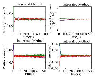
Based on a combination of the measurements from feature points (D1,D3),lines (
|
Figure 4 Estimation errors of the method using feature points,lines and circles |
|
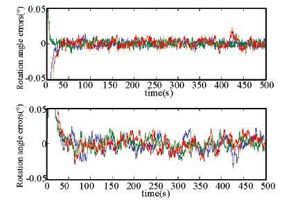
Figure 5 Rotation angle estimation errors for circles in the integrated method |
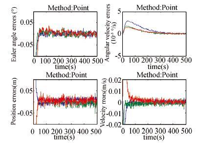
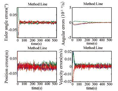
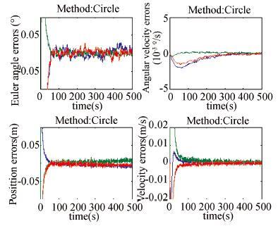
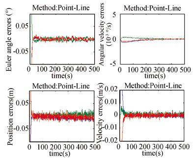
To compare the performance of the proposed integrated estimation algorithm with other combinations of the features,the following cases are considered: 1) Use point features only (D1,D2,D3,D4); 2) Use line features only (
|
Figure 6 Estimation errors of the method using feature points |
|
Figure 7 Estimation errors of the method using feature lines |
|
Figure 8 Estimation errors of the method using feature circles |
|
Figure 9 Estimation errors of the method using feature points and lines |
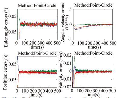
|
Figure 10 Estimation errors of the method using feature points and circles |
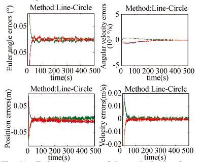
|
Figure 11 Estimation errors of the method using feature lines and circles |
| Table 1 Estimation errors using different combinations of geometric features |
In order to validate the proposed method in the case of lager initial errors,the initial guess of the estimation is given as
| $\begin{align} & {{{\tilde{q}}}_{fl,P}}\left( 0 \right)={{\left[ 0.919\text{ }7,0.026\text{ }5,0.065\text{ }4,0.386\text{ }1 \right]}^{\text{T}}} \\ & \tilde{r}_{fl,P}^{fP}\left( 0 \right)={{\left[ -60,80,100 \right]}^{\text{T}}}\text{m,}\tilde{\hat{\omega }}_{fl,P}^{fP}\left( 0 \right)=\hat{0} \\ \end{align}$ |
The simulation results are shown in Fig. 12,which validate the effectiveness of the proposed estimation method in the case of lager initial errors. However,the larger initial estimation errors cost longer time to converge and the estimation convergence errors become larger. To improve the performance of the estimation,the author considers employing other advanced filtering algorithms such as the Unscented Kalman Filter (UKF) and Partical Fliter (PF),and it will be the direction for the future research.
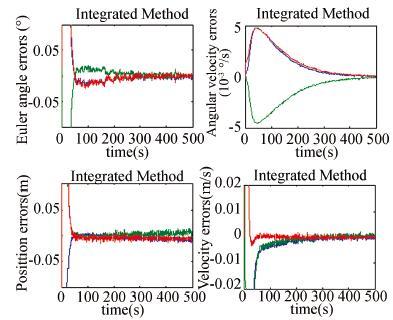
|
Figure 12 stimation errors of the method using feature lines and circles (larger initial estimation errors) |
6 Conclusions
By employing dual numbers,an integrated observation model is developed based on a combination of multiple geometric features including points,lines and circles. In addition,a six-degree-of-freedom relative motion model is derived,which can describe the rotation-translation coupling effect due to the points deviating from the center of the mass. Based on the proposed relative dynamics and the integrated observation model,Extended Kalman Filter is presented to estimate the relative state between spacecraft. Finally,numerical simulations are provided to illustrate the effectiveness of the proposed algorithms. The simulation results demonstrate that high accuracy can be achieved by using the presented estimation technique,and by comparing with other algorithms using different combinations of features,the integrated technique yields a superior estimation accuracy and fastest convergence rate.
| [1] |
Segal S, Gurfil P. Stereoscopic vision-based spacecraft relative state estimation.
AIAA Guidance, Navigation, and Control Conference.AIAA,2009 : 2009-6094.
( 0) 0)
|
| [2] |
Alfriend K T, Vadali S R, Gurfil P, et al. Spacecraft formation flying-dynamics, control and navigation.
Elsevier Astrodynamics Series,2010 : 1-8.
( 0) 0)
|
| [3] |
Subbarao K, Welsh S. Nonlinear control of motion synchronization for satellite proximity operations.
Journal of Guidance,Control and Dynamics,2008, 31 (5) : 1284-1294.
( 0) 0)
|
| [4] |
Segal S, Gurfil P. Effect of Kinematic rotation-translation coupling on relative spacecraft translational dynamics.
Journal of Guidance,Control and Dynamics,2009, 32 (3) : 1045-1050.
( 0) 0)
|
| [5] |
Pan H, Kapila V. Adaptive nonlinear control for spacecraft formation flying with coupled translational and attitude dynamics.
Proceedings of 40th IEEE Conference on Decision and Control. New York,2001 : 2057-2062.
( 0) 0)
|
| [6] |
Kristiansen R, Nicklasson P J, Gravdahl J T. Spacecraft coordination control in 6DOF:integrator backstepping vs passivity-based control.
Automatica,2008, 44 (11) : 2896-2901.
( 0) 0)
|
| [7] |
Clifford W K. Preliminary sketch of bi-quaternions.
Proc. London Mathematics Society,1873, 1 : 381-395.
( 0) 0)
|
| [8] |
Brodsky V, Shoham M. Dual numbers representation of rigid body dynamics.
Mechanism and Machine Theory,1999, 34 (5) : 693-718.
( 0) 0)
|
| [9] |
Wu Y, Hu X, Hu D, et al. Strapdown inertial navigation system algorithms based on dual quaternions.
IEEE Transactions on Aerospace and Electronic Systems,2005, 41 (1) : 110-132.
( 0) 0)
|
| [10] |
Gan D, Liao Q, Wei S, et al. Dual quaternion-based inverse Kinematics of the general spatial 7R mechanism.
Proceedings of the Institution of Mechanical Engineering Science, Part C: Journal of Mechanical Engineering Science,2008, 222 (8) : 1593-1598.
( 0) 0)
|
| [11] |
Alba Perez, McCarthy J M. Dual quaternion synthesis of constrained robotic systems.
Journal of Mechanical Design,2004, 126 (3) : 425-435.
( 0) 0)
|
| [12] |
Han D, Wei Q, Li Z, et al. Control of oriented mechanical systems: a method based on dual quaternion.
Proceedings of the 17th World Congress the International Federation of automatic Control. Seoul,2008 : 3836-3841.
( 0) 0)
|
| [13] |
Wang J, Liang H, Sun Z, et al. Finite-time control for spacecraft formation with dual-number-based description.
Journal of Guidance, Control and Dynamics,2012, 35 (3) : 950-962.
( 0) 0)
|
| [14] |
Bertozzi M, Broggi A, Fascioli A. Vision-based intelligent vehicles: state of the art and perspectives.
Robotics and Autonomous Systems,2000, 32 : 1-16.
( 0) 0)
|
| [15] |
Segal S, Carmi A, Gurfil P. Vision-based relative state estimation of non-cooperative spacecraft under modeling uncertainty.
Proceedings of the IEEE Aerospace Conference. Big Sky,2011 : 1-8.
( 0) 0)
|
| [16] |
Tsai R. A versatile camera calibration technique for high-accuracy 3D machine vision metrology using off-the-shelf TV cameras and lens.
IEEE Journal of Robotics and Automation,1987, 3 : 223-244.
( 0) 0)
|
| [17] |
Holt R J, Netravali A N. Camera calibration problem: some new results.
Computer Vision, Graphics, and Image Processing,1991, 54 (3) : 368-383.
( 0) 0)
|
| [18] |
Kim S G, Crassidis J L, Cheng Y, et al. Kalman filtering for relative spacecraft attitude and position estimation.
Journal of Guidance, Control and Dynamics,2007, 30 (1) : 133-143.
( 0) 0)
|
| [19] |
Xing Y, Cao X, Zhang S, et al. Relative position and attitude estimation for satellite formation with coupled translational and rotational dynamics.
ACTA Astronautica,2010, 67 : 455-467.
( 0) 0)
|
| [20] |
Chen S Y, Tsai W H. Systematic approach to analytic determination of camera parameters by line features.
Pattern Recognition,1990, 23 (8) : 859-897.
( 0) 0)
|
| [21] |
Liu Y, Huang T, Faugeras O D. Determination of camera locations from 2d to 3d Line and point correspondence.
IEEE Transactions on Pattern Analysis and Machine Intelligence,1990, 12 (1) : 28-37.
( 0) 0)
|
| [22] |
Chiang Y T, Huang P Y, Chen H W, et al. Estimation of 3-D transformation from 2-D observing image using dual quaternion.
Proceedings of 17th World Congress, the International Federation of Automatic Control. Seoul,2008 : 10445-10450.
( 0) 0)
|
| [23] |
Goddard J S. Pose and motion estimation from vision using dual quaternion-based extended Kalman filtering. The University of Tennessee, Knoxville, Tennessee, 1997.
( 0) 0)
|
| [24] |
Song D M. Conics-based stereo,motion estimation, and pose determination.
International Journal of Computer Vision,1993, 10 (1) : 7-25.
( 0) 0)
|
 2016, Vol. 23


