The lime rotary kiln is key equipment in metallurgical industry. The running state of rotary kiln influences the quality of the products, energy consumption, safety and cost directly[1]. The calcination zone temperature of lime rotary kiln is an important parameter which can reflect the running state of rotary kiln, and it plays a decisive role that can guarantee the quality of products, achieve safe and stable operation of the rotary kiln and reduce labor intensity.The good control performance of calcination temperature can ensure the roasting effect of material, and guarantee the full chemical reaction [2].
With the development of new intelligent modeling and control methods, a large number of intelligent modeling methods are successfully applied on the process of rotary kiln modeling. Li et al. [3] proposed a modeling method based on extreme learning machine (ELM), and obtained the good running effect in practical field applications. In his doctoral dissertation, Georgallis[4] gave a detailed description on three-dimensional lime rotary kiln model based on material flow and heat transfer.Söğüt[5] built a rotary kiln mathematical model for thermal recovery process [5]. Mathematical model has been developed by using finite element technique to track the reaction front movement from the surface to the core in Ref.[6], temperature profiles inside the lime particle are calculated and the influence of the reaction front position on these temperature profiles has been analyzed. Zhang et al. [7] proposed modeling method based on subspace identification for lime kiln calcination process. The simulation results show that this model is of high accuracy for describing the characteristics of lime kiln calcination process. For the purpose of obtaining the accurate soft-sensing model in case the data are less with the temperature similarity between kiln head and calcination zone taken into consideration, the process modeling based on process similarity is introduced [8]. Simulation results verified the effectiveness of this modeling method. A highly effective moisture sensing and control system based on sensing and controlling mud moisture is proposed in Ref.[9], it has been validated by numerous applications. The modeling for calcination zone temperature of rotary kiln has many mature experiences after the long-term development, but until today there are some problems, such as, difficult to model accurately, too much constrained conditions, and not universal properties.
The intelligent control is the main research topic of rotary kiln temperature control, include fuzzy control[10], neural network [11-13], expert system[14-15]and hybrid intelligent control strategy [16-18], etc. But the rotary kiln calcination zone temperature control is a complex control system. The production process of lime rotary kiln is a complicated physical chemistry course of reaction and has characteristics of big inertia, pure time-delay, nonlinearity and etc. So the calcination zone temperature modeling of rotary kiln is not easy to be set up by traditional methods. On the other hand, rotary kiln has the feature of complicated circumstances and variety of parameters, higher calcination zone temperature controller is needed. And it is difficult to control the calcination zone temperature by traditional methods. In order to realize the automatic control with effectively and precisely, only using single control method can not achieve the expected control performance.
In one word, the rotary kiln calcination zone temperature control includes two core parts: The first is how to model accurately. The whole rotary kiln is a nonlinear system between input control variable and output temperature.The second is how to choose an effective control strategy which can suppress the interference and noise and guarantee the stability of control system. This paper will carry out the study on these two issues.
The rotary kiln calcination zone temperature is regarded as the controlled object in this paper. Least square support vector machine (LSSVM) has good capability of nonlinear mapping, need small sample data, and this paper will utilize LSSVM to build the nonlinear model for rotary kiln calcination zone temperature. The input and output training data in this paper come from actual production field. At the same time, because the built model is nonlinear, the rolling optimization of control variable is a nonlinear constraint problem. This paper proposes an improved harmony search (IHS) algorithm for iterative optimization of control variable. At each sampled moment, LSSVM model can predict the rotary kiln calcination zone temperature of future moment, the fitness function about control variable and error can be obtained through error correction of output feedback. The IHS algorithm is used as the rolling optimization strategy for the calculation of control variable. The simulation results show that this control method is effective.
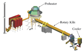
2 The Controlled Object DescriptionA lime rotary kiln system has many technological processes. The process can be mainly divided into material system and air flow system. The raw material changes into product after preheating, high temperature calcination and cooling.Primary air, secondary air and coke oven gas constitute the air flow system. Secondary air is used to cool the finished product. The waste gas enters preheater and preheats for raw material.The whole technological process is shown in Fig. 1[15].
|
Figure 1 Technological process chart of rotary kiln |
Calcination temperature in the rotary kiln is an important process parameter that plays a decisive role to ensure product quality. The lime kiln under study is 600 ton/d, 4.0 m×60 m. The main factor that affects the quality of lime rotary kiln is calcination zone temperature. The ideal temperature range is between 1 200-1 300 ℃.
There are many factors which affect the calcination temperature in the rotary kiln, such as raw material flow, gas flow, rotary kiln speed and other random disturbances. These factors can be described as follows.
1) The raw material flow affects the calcination effect in rotary kiln. The more raw materials per unit time in the kiln are, the thicker the thickness of kiln material layer is. It will lead the calcination process not sufficient, and then affect the quality of clinker.
2) The gas flow, premise condition for the stability of the calcination zone temperature is the good control of the gas flow. According to the different characteristic of rotary kiln, the appropriate gas flow should be determined.
3) The secondary air has also a great influence on the calcination zone temperature. If air quantity is insufficient, it leads less heat, fuel waste, and will affect the smooth progress of the reaction. If air quantity is too much, it can also take away a lot of heat, reduce the temperature inside the kiln, and can also cause the energy waste. So it is necessary to maintain the secondary air flow at a proper level.
4) The rotary kiln speed directly influences the time of the material in the whole cylinder, and indirectly influences the production and quality of the clinker. If the rotation speed of the rotary kiln is too fast, the residence time of the material in the calcination zone is less than the required time for the reaction. And if the rotary kiln is too slow and the material stay time in the kiln is too long, the system capacity and efficiency is reduced.
5) Random disturbances are many disturbances of rotary kiln. The whole system is inevitable, so under a certain disturbance, the system should be able to return to a stable temperature range within the shortest possible time, which can ensure the quality of clinker, require the dynamic response of the system to be fast, and adjust time to be short.
In practical applications, the calcination zone temperature is the result of fuels burning, so the gas flow can be seen as determinant variables influence the calcination zone temperature. The raw material flow is determined by the push rod time of preheater. So the push rod time is another key control variable. The other factors, such as rotary kiln speed and secondary air flow, they are generally constant value. The random disturbances are always uncontrollable in the actual application. So in this paper, the gas flow and push rod time are chosen as control variables.
3 LSSVM Modeling for Calcination Zone TemperatureLSSVM uses a nonlinear mapping function ϕ(·). The sample space is mapped into a high-dimensional or even infinite dimensional feature space through this function [19]. In this feature space, there is f(x)=wTϕ(x)+b, where w is weight coefficient vector; b is a constant bias. Optimal w and b can be obtained by minimizing the objective function expressed as following equation.
| $\begin{array}{l} \mathop {\min }\limits_{\boldsymbol{w},b,e} J\left( {\boldsymbol{w,e}} \right) = \frac{1}{2}{\left\| \boldsymbol{w} \right\|^2} + \frac{1}{2}\gamma \sum\limits_{k = 1}^N {e_k^2} \\ {\rm{s}}{\rm{.t}}{\rm{.}}\;{y_k} = {\boldsymbol{w}^{\rm{T}}}\phi \left( {{\boldsymbol{x}_k}} \right) + b + {e_k},k = 1,2, \cdots ,N \end{array}$ | (1) |
Lagrange function is established for solving constrained optimization problems:
| $\begin{array}{c} L\left( {\boldsymbol{w},b,e,\alpha } \right) = J\left( {\boldsymbol{w},e} \right) - \sum\limits_{k = 1}^N {{\alpha _k}\left\{ {{\boldsymbol{w}^{\rm{T}}}\phi \left( {{\boldsymbol{x}_k}} \right) + } \right.} \\ \left. {b + {e_k} - {y_k}} \right\} \end{array}$ | (2) |
Where αk is a Lagrange multiplier. The Lagrange function can be used for solving extreme value. The above optimization problem is transformed into solving the linear equations.
According to Mercer conditions, the presence of mapping function ϕ(·) and kernel function K(·) satisfy the following equation:
| $K\left( {{\boldsymbol{x}_{\rm{i}}},{\boldsymbol{x}_{\rm{j}}}} \right) = \phi = {\left( {{\boldsymbol{x}_{\rm{i}}}} \right)^{\rm{T}}}\phi \left( {{\boldsymbol{x}_j}} \right)$ | (3) |
Nonlinear mapping ability of LSSVM prediction model is determined by the kernel function. Kernel function is used for solving the LSSVM prediction model samples mapping from input space to output feature space. Therefore, different kernel functions have different learning abilities and generalization abilities. The most widely used is radial basis function (RBF) kernel, which is applicable for low-dimensional, high-dimensional, small sample, large sample and other problems. The RBF kernel is expressed as Eq. (4).
| $\boldsymbol{y} = \sum\limits_{i = 1}^N {{\alpha _i}K\left( {{\boldsymbol{x}_i},{\boldsymbol{x}_j}} \right)} + b$ | (4) |
Where σ2 is the width of RBF kernel function. The predictive value of LSSVM model is
| $\begin{array}{c} y\left( k \right) = f\left( {y\left( {k - 1} \right), \cdots ,y\left( {k - n} \right),{u_1}\left( k \right), \cdots ,{u_1} - m} \right),\\ \left. { \cdots ,{u_j}\left( k \right), \cdots ,{u_j}\left( {k - m} \right)} \right),y,u \in {{\rm{\boldsymbol{R}}}^n} \end{array}$ | (5) |
Rotary kiln production is a typical nonlinear process, and it is difficult to establish the mathematical model. The LSSVM regression model can be established through the following nonlinear system:
| $\begin{array}{l} {y_k} = f\left( {y\left( {k - 1} \right), \cdots ,y\left( {k - n} \right),{u_1}\left( k \right), \cdots ,{u_1}\left( {k - m} \right),} \right.\\ \cdots ,{u_j}\left( k \right), \cdots ,{u_j}\left( {k - m} \right),y,u \in {{\rm{\boldsymbol{R}}}^n} \end{array}$ | (6) |
Where y(k) is rotary kiln control system output at moment k, that is the calcination zone temperature. f(·) is nonlinear mapping function about the rotary kiln production process system output value. u=(u1, u2, …, um) is control variables. The system input U(k)=(u(k), u(k-1), …, u(k-m)) and system output Y(k)=(y(k-1), y(k-2), …, y(k-n)) is chosen as input vector of LSSVM model, then training sample sets are expressed as (X(k), Y(k)).
In this paper, the output vector Y is the calcination zone temperature. Because the control variables are gas flow and push rod time, these two parameters are chosen as U, therefore, input vector X(k) include the calcination zone temperature y(k) and control variable vector U(k). In this paper, considering the control precision and computing time, n is determined as 4, and m is determined as 2. The input and output vectors of the LSSVM model are as follows.
| $\begin{array}{c} \boldsymbol{X}\left( k \right) = \left[ {\begin{array}{*{20}{c}} {y\left( {k - 1} \right)}&{y\left( {k - 2} \right)}&{y\left( {k - 3} \right)}&{y\left( {k - 4} \right)}&{{u_1}\left( k \right)} \end{array}} \right.\\ {\left. {\begin{array}{*{20}{c}} {{u_2}\left( k \right)}&{{u_2}\left( k \right)}&{{u_2}\left( {k - 1} \right)}&{{u_1}\left( {k - 2} \right)}&{{u_2}\left( {k - 2} \right)} \end{array}} \right]^{\rm{T}}} \end{array}$ | (7) |
| $\boldsymbol{Y}\left( k \right) = \left[ {y\left( k \right)} \right]$ | (8) |
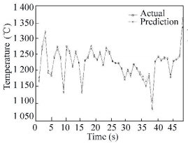
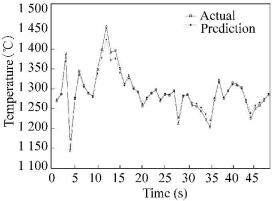
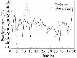
Because the modeling process of LSSVM needs small sample data, 148 group data from a lime rotary kiln factory in Hebei Province of China are collected. The former 100 group data are used as training sample set, and the latter 48 group data are used as the test sample set. The cross and verification method is used for parameters optimization of LSSVM model. The optimization results are: the regularization parameter γ is 4.22, and kernel function width σ2 is 0.02. Fig. 2 shows the comparison curves between actual and predictive value of training sample set. Fig. 3 shows the comparison curves between actual and predictive value of testing sample set. Fig. 4 shows the predictive error of training and testing sample set. From these figures, it can be known that the built prediction model has good prediction effect. Table 1 gives the maximum absolute error, least absolute error, root mean square error (RMSE), mean absolute percentage error (MAPE) of training and testing sample test. From Table 1, it can be known that the built model has smaller predictive error. This model can meet the needs of modeling accuracy.
|
Figure 2 Comparison result of training sample |
|
Figure 3 Comparison result of testing sample |
|
Figure 4 Error of training and testing sample |
| Table 1 Modeling error |
4 IHS Algorithm 4.1 The Standard HS Algorithm
Harmony search (HS) algorithm is a swarm intelligence optimization algorithm, which was proposed in 2001[20]. HS algorithm comes from the music creative process. The standard HS algorithm uses all individuals cooperate to produce a new individual; it does not depend on the initial conditions. HS algorithm has a simple structure; it is easy to implement with fast convergence characteristics. The relevant Ref.[21] shows that optimization performance of harmony search algorithm is better than genetic algorithms and simulated annealing algorithm and other optimization algorithms. The HS algorithm is widely applied to optimize many practical problems [22-25].
The following parts are the optimization process of standard harmony search algorithm. For a given optimization problem:
| $\begin{array}{l} \min f\left( X \right)\\ {\rm{s}}{\rm{.t}}{\rm{.}}\;\;{x_i} \in \left[{{L_i}, {U_i}} \right] \end{array}$ |
Where X is a real-valued vector with u dimensions; f(X) is a real continuous function.
Step 1 Initialization parameters of HS algorithm are as follows: harmony memory size (HMS), harmony memory consideration rate (HMCR), pitch adjusting rate (PAR), band width (BW), number of iteration (NI), the range of the decision variables is [Li, Ui].
Step 2 Creating a harmony memory randomly as follows:
| $\boldsymbol{HM} = \left[ {\begin{array}{*{20}{c}} {{\boldsymbol{X}_1}}\\ {{\boldsymbol{X}_2}}\\ \vdots \\ {{\boldsymbol{X}_m}} \end{array}} \right] = \left[ {\begin{array}{*{20}{c}} {{x_{11}}}&{{x_{12}}}& \cdots &{{x_{1{\rm{n}}}}}\\ {{x_{21}}}&{{x_{22}}}& \cdots &{{x_{2{\rm{n}}}}}\\ \vdots & \vdots & \vdots & \vdots \\ {{x_{{\rm{m}}1}}}&{{x_{{\rm{m}}2}}}& \cdots &{{x_{{\rm{mn}}}}} \end{array}} \right];m = HMS$ | (9) |
Step 3 Producing a candidate solution, Xnew=(xnew(1), xnew(1), ···, xnew(j)), xnew(j) is generated by the following steps:
| ${x_{{\rm{new}}}}\left( j \right) = \left\{ \begin{array}{l} {x_{md\left( i \right),j}}\;\;\;\;\;\;\;\;\;\;\;\;\;\;\;\;\;\;\;{r_1} < HMCR\\ {x_{{\rm{new}}}}\left( j \right) \in \left[ {{L_i},{U_i}} \right]\;\;\;{\rm{others}} \end{array} \right.$ | (10) |
Where xmd(i), j is a j-th row component of the harmony memory with randomly; xnew(j)is a random value of the j-th variable; r1 is a random number uniformly distributed between [0, 1]. Then, if xnew(j)is the solution of the components which is selected from harmony memory, xnew(j) will be trimmed as next equation:
| ${x_{{\rm{new}}}}\left( j \right) = \left\{ \begin{array}{l} {x_{{\rm{new}}}}\left( j \right) \pm {r_3} \times BW,\;\;\;{r_2} < PAR\\ {x_{{\rm{new}}}}\left( j \right),\;\;\;\;\;\;\;\;\;\;\;\;\;\;\;\;{\rm{others}} \end{array} \right.$ | (11) |
Where r2 and r3 are random number which uniformly distributed between [0, 1];
Step 4 Updating the harmony memory, if f(Xnew) < f(Xw), and X is the worst solution in the harmony memory, then Xw=Xnew;
Step 5 Repeat Steps 3 and 4, until the number of iterations are reached NI.
4.2 Improved HS AlgorithmFrom the standard harmony search algorithm, it can be seen that HMCR and PAR can help the algorithm find global and local best solutions. PAR and BW are two very important parameters in harmony search process. In the early of optimization process, a smaller PAR value and larger BW value are conducive to enhance the diversity of the solution vector, which can quickly find local optimal value. However, in the later of optimization process, the smaller BW and larger PAR value is conducive to find the global optimal solution quickly. Standard harmony search algorithm uses a fixed parameter values, but it does not consider the requirements of local optimal solution and the global optimal solution. Meanwhile, the search speed and convergence accuracy of harmony algorithm are related to these key parameters. In order to improve the search efficiency of the algorithm and overcome the shortcomings of standard harmony search algorithm, some improvements for HS algorithm are proposed in this paper.
For the parameter HMCR, it should be dynamically adjusted from big to small. This causes the harmony search algorithm first full search in harmony memory, and then transferred to the external harmony memory in the later of iterations. It can increase the diversity of population. Adjustment method of HMCR in this paper is as follows:
| $\begin{array}{l} HMCR\left( t \right) = HMCR\left( {t - 1} \right) \times \rho \\ {\rm{s}}{\rm{.t}}{\rm{.}}HMCR\left( t \right) \in \left[ {HMC{R_{\min }},HMC{R_{\max }}} \right] \end{array}$ | (12) |
In the early of harmony search algorithm, the smaller PAR is good for the algorithm which can search in the better regional. In the later of harmony search algorithm, the larger PAR can help algorithm jump out of local optimum value, so the PAR value should be changed from small to large. The changes of PAR in this paper are as follows:
| $PAR\left( t \right) = \frac{{PA{R_{\max }} - PA{R_{\min }}}}{{\sqrt {NI} }} \times \sqrt t + PA{R_{\min }}$ | (13) |
For the parameter BW, in the early of the algorithm, the bigger BW is good for the algorithm which can search in a wide range. In the later of the algorithm search process, the smaller BW will help harmony search algorithm which has precise search within a small range. So the changing of BW value should be from small to large, the changes of BW in this paper are as follows:
| $BW\left( t \right) = B{W_{\min }} + \left( {B{W_{\max }} - B{W_{\min }}} \right) \times {e^{ - t}}$ | (14) |
When standard harmony search algorithm is updating memory, new solution xnew is generated by selecting a component from the memory randomly. This operation will cause many problems for algorithm search process, such as search direction uncertain with randomness. This paper refers to the crossover operation idea of genetic algorithm, and a new solution xnew1 is generated according to the standard harmony search algorithm, and then according to Eq. (15), the second new solution xnew2 is generated through xnew1 cross operation with another column component xnew.
| ${x_{{\rm{new2}}}} = u{x_{{\rm{new}}1}} + \left( {1 - u} \right){x_{{\rm{new}}}}$ | (15) |
Where u is a scale factor. If f(xnew1) < f(xnew2), reserved xnew1, if not, reserved xnew2, this will keep the search direction certainty.
In order to verify the performance of IHS algorithm proposed in this paper, the Sphere function is used as testing function. The expression of Sphere function is:
| $f = \sum\limits_{i = 1}^n {x_i^2,{x_i} \in \left[ { - 100,100} \right]} $ | (16) |
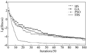
The standard HS algorithm parameters are:HMCR=0.9, PAR=0.3, BW=0.01, HMS=6, IHS algorithm parameters are HMCRmax=1, HMCRmin=0.4, ρ=0.97, PARmax=0.9, PARmin=0.4, BWmin=0.000 1, BWmax=1, HMS=6, cross-factor u is 0.8, the iterations of HS and IHS is chosen as 5 000. The numbers of variable xi are 4. In order to compare the optimization performance of the algorithm, genetic algorithm (GA) and particle swarm optimization (PSO) algorithm is added for the comparison of optimization ability. The GA parameters are: population quantity is 20, and evolutionary algebra is 5 000, and the crossover probability is 0.8, and mutation probability is 0.2. The PSO parameters are: learning factor c1 is 1.5 and c2 is 1.7, and the inertia weight is 1, and evolutionary algebra is 5 000.
Fig. 5 shows fitness convergence curve. For the convenience of display, the horizontal ordinate is the number of iterations divided by 50; the vertical ordinate is the fitness takes on logarithm of 10. It can be seen that the improved HS algorithm in this paper is better than the standard HS, GA and PSO algorithm. Table 2 gives the compare result of HS and other algorithms, which include optimization results and the best fitness value.
|
Figure 5 Fitness convergence curve of Sphere function |
| Table 2 Comparison results of IHS and other algorithms |
The simulation results on Sphere function verified IHS algorithm has better convergence speed and precision than standard HS, GA and PSO algorithm. In the next sections, IHS algorithm will be used for control variables optimization in LSSVM predictive control process.
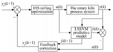
5 LSSVM Predictive Control with IHS Algorithm 5.1 Predictive Control AlgorithmAssuming that LSSVM is built as the model of calcination zone temperature of rotary kiln, and this nonlinear model is shown as Eq.(5).The input control value is u(k), and the system output value is y(k), and the system output estimated value ŷ(k) can be obtained through LSSVM prediction model. However, due to noise or model mismatch and other reasons, there is output error between the system predicted value ŷ(k) and actual output value y(k). The predictive error at k time is:
| $\boldsymbol{e}\left( k \right) = \boldsymbol{y}\left( k \right) - \boldsymbol{\hat y}\left( k \right)$ | (17) |
The correction value can be obtained by error correction ŷ(k+1):
| ${\boldsymbol{y}_p}\left( {k + 1} \right) = \boldsymbol{\hat y}\left( {k + 1} \right) + \boldsymbol{e}\left( k \right)$ | (18) |
The control problem of rotary kiln calcination zone temperature is to find the minimum objective function by IHS algorithm. For a nonlinear system expressed as Eq. (6), the quadratic performance index is the typical performance function of nonlinear model predictive control (NMPC) problem. For control problems, the future m control increments at start time k should make the future n output predicted value track the expected value as far as possible. There are two questions be considered. The deviation or squared deviation between predicted and expected value is minimum. The rotary kiln discussed in this paper has two inputs and one output. This paper determines the fitness function of control value u(k) as the following Eq. (19).
| $\begin{array}{l} \min J = E\left\{ {q{{\left[ {\sum\limits_{i = 1}^4 {{y_r}\left( {k + i} \right) - {y_p}\left( {k + i} \right)} } \right]}^2} + } \right.\\ \left. {\sum\limits_{j = 1}^2 {{\lambda _j}{{\left[ {u\left( {k + j} \right) - u\left( k \right)} \right]}^2}} } \right\} \end{array}$ | (19) |
Where E represents mathematics expectation; yr(k) is the reference trajectory at time k; yp(k) is predictive output value by the feedback correction at time k; q and λj are weighting coefficients. IHS algorithm is used for optimization control of the calcination zone temperature. The predictive control system diagram of rotary kiln in this paper is shown in Fig. 6.
|
Figure 6 Structure of LSSVM predictive control with IHS |
The LSSVM predictive control for calcination zone temperature in rotary kiln with IHS algorithm in this paper can be described as follows:
Step 1 Set IHS algorithm (HMCRmax, HMCRmin, ρ, PARmax, PARmin, BWmin, BWmax, HMS and u) and LSSVM model parameters (γ and σ2).
Step 2 The input and output sampling data are obtained through nonlinear systems of lime rotary kiln calcining process. LSSVM is used for the training of sample data, the rotary kiln calcination zone temperature prediction model based on LSSVM model is established offline.
Step 3 The certain control value sequence u(k) and system output is y(k) at time k, and then the predicted output ŷ(k) can be obtained through LSSVM prediction model, the output predicted value ŷ(k+1) through control value u(k+1) to be optimized at the next time, the fitness of the objective function is calculated.
Step 4 The control value u(k+1) at the next time is regarded as the optimization object of IHS algorithm. The optimal control value u(k+1) can be obtained by rolling optimization of objective function.
Step 5 The optimal control value u(k+1) is applied to the lime kiln control system, let k=k+1, go to step 5, until the simulation is finished.
5.2 Stability Analysis of AlgorithmsAssuming Jk is the objective function of k-th optimization process. Eq. (19) shows Jk≥0.If k→∞, the system is stable when Jk=J∞=0. If J∞=0, it can be known ypi(∞)=yri(∞) by Eq.(19), that is to say, the system output is equal to the desired output. It is only need to prove J∞=0 when k→∞, and then the system is asymptotically stable.
Using reduction to absurdity, assuming k→∞ there is J∞≠0, it is can be seen Jk is monotone decreasing function by IHS algorithm, at time k, there is:
| $\Delta {J_k} = {J_{k + 1}} - {J_k} < 0,{J_\infty } \le {J_k} \le {J_0}$ | (20) |
J0 is object fitness function value at initial time and it is a constant value. Obviously Jk is a bounded closed set. It can be known that ΔJk have maximum value from the Weierstrass theorem. Let the maximum value of ΔJk be ΔJmax, because J∞≠0 and object fitness function is non-negative, there is ΔJmax≠0, and Jk is transformed into the following form:
| ${J_k} = {J_0} + \sum\limits_{t = 0}^{k - 1} {\Delta {J_t} \le {J_0} - k\Delta {J_{\max }}} $ | (21) |
Because of-ΔJmax < 0, the above equation indicate that J∞→-∞ when k→∞, obviously, it is conflict with the objective fitness function is non-negative, therefore it is J∞=0.
From the above proof process, it shows the control system of this paper is asymptotically stable.
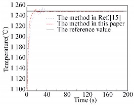
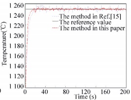
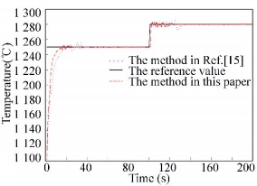
6 Simulation and VerificationIn order to verify the effectiveness of the control method proposed in this paper, this section will use the above proposed predictive control method to realize the control for calcination zone temperature of rotary kiln. The parameters of IHS algorithm are as follows: HMCRmax=1, HMCRmin=0.4, ρ=0.97, PARmax=0.9, PARmin=0.4, BWmin=0.000 1, BWmax=1, HMS=6, the maximum number of iterations as 100. The push rod time of rotary kiln is set to belong to [15, 40], and gas flow range is belong to [8 500, 9 500], the maximum output temperature value ymax=1 300, the minimum output temperature value ymin=1 100, and the input reference trajectory is a step signal with amplitude as 1 250, and initial calcinations zone temperature value is set to 1 100. The control method in Ref.[15] is compared. Fig. 7 shows the system output response curve. In order to verify the anti-interference ability of the predictive control method in this paper, the random white noise signal is added in the output with amplitude as 10. Fig. 8 shows the system output response under output interference. In order to verify the performance of the following changed reference value of the proposed method, the reference value is changed to 1 270 at the 100th sampling time. Fig. 9 represents the system output response when the reference value changed.
|
Figure 7 System step response curve |
|
Figure 8 System output response under interference |
|
Figure 9 System response curve when reference value changed |
As shown in Figs. 7-9, the control method proposed in this paper can track the reference output value of the calcination zone temperature with fast and stable. At the same time, the output of the system under disturbance or reference value changed can also better track the reference value, so LSSVM predictive control for calcination zone temperature in rotary kiln with IHS algorithm has good adaptive ability and robustness. The simulation results have shown that for the time varying and nonlinear lime rotary kiln control object. The control strategy proposed in this paper can not only control burning temperature to achieve the desired target value, but also has the robust and fast tracking ability. The model predictive control (MPC) method is used in Ref.[15], which needs a large amount of matrix computation. The control variable obtained from MPC may be not the optimal value. Compared with the method in Ref.[15], the method in this paper has better control performance. The reason for the performance improvement is LSSVM used in this paper has good nonlinear mapping ability. The calcinations zone temperature prediction model built in this paper can reflect the actual characteristics of the rotary kiln system. The other reason is IHS algorithm has good convergence characteristics and optimization abilities, which can find the optimal and suitable control variable for the control system. The appropriate control variable can be applied to the controlled rotary kiln object at each sampling moment.
On the other hand, the rolling optimization time of control variables is measured, 200 simulation sampling cycle need 50.65 s, so the average time of one step rolling optimization of control value is about 0.25 s, The average computation time of method in Ref.[15] is 0.57 s under the same simulation conditions.The main reason of computation time reduced is the rolling optimization in this paper does not need the complex matrix computation.This predictive control method obviously can be applied to actual control applications.
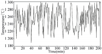
Fig. 10 shows the control effect in the actual applications. The control system is realized by Visual C++ and Matlab 2010b. From Fig. 10, it can be seen that the control method in this paper can be used in actual production process, and maintain the temperature near the setting value (the control error belongs to positive and negative 50 ℃).
|
Figure 10 The control effect in actual applications 7 Conclusions |
1) In this paper, the lime rotary kiln calcination zone temperature is used as the controlled object, and a LSSVM predictive control for calcination zone temperature with IHS algorithm is proposed. The input and output data are utilized to build nonlinear predictive model of rotary kiln calcination zone temperature through LSSVM model. An improved harmony search algorithm is presented for rolling optimization of optimal control value. The simulation and actual experimental results show the effectiveness of this method.
2) In the simulation of the paper, the parameters of IHS algorithm are the same with Section 4.2. Because IHS algorithm obtained better performance with these parameters, the paper uses the same parameters. In the future research work, the authors will test the effect of other parameters on the control effect.
| [1] |
Wang C B, Chen L, Jia L F, et al. Simultaneous calcination and sulfation of limestone in CFBB.
Applied Energy, 2015 , 155 : 478-484.
DOI:10.1016/j.apenergy.2015.05.070 ( 0) 0)
|
| [2] |
Saidur R, Hossain M S, Islam M R, et al. A review on kiln system modeling.
Renewable and Sustainable Energy Reviews, 2011 , 15 (5) : 2487-2500.
DOI:10.1016/j.rser.2011.01.020 ( 0) 0)
|
| [3] |
Li W T, Wang D H, Chai T Y. Burning state recognition of rotary kiln using ELMs with heterogeneous features.
Neurocomputing, 2013 , 102 : 144-153.
DOI:10.1016/j.neucom.2011.12.047 ( 0) 0)
|
| [4] |
Georgallis M.
Mathematical modelling of lime kilns. Vancouver: University of British Columbia, 2004 .
( 0) 0)
|
| [5] |
Söğüt Z, Oktay Z, Karakoç H. Mathematical modeling of heat recovery from a rotary kiln.
Applied Thermal Engineering, 2010 , 30 (8/9) : 817-825.
DOI:10.1016/j.applthermaleng.2009.12.009 ( 0) 0)
|
| [6] |
Sandaka P C G, Nallathambi A K, Specht E, et al. Finite element analysis of reaction front tracking in lime calcination.Proceedings of ASME/JSME 2011 8th Thermal Engineering Joint Conference(AJTEC 2011). New York:American Society of Mechanical Engineers, 2011. T10130-T10130-6.
( 0) 0)
|
| [7] |
Zhang L, Gao B, Bao Z J. Modeling Method based on subspace identification for lime kiln calcination process. Proceedings of 4th International Conference on Mechanical and Electrical Technology(ICMET 2012). Clausthal-Zellerfeld:Trans Tech Publications, 2012. 1882-1885.
( 0) 0)
|
| [8] |
Zhang Li, Gao Xianwen, Wang Jiesheng, et al. Soft-sensing for calcining zone temperature in rotary kiln based on model migration.
Journal of Northeastern University:Natural Science, 2011 , 32 (2) : 175-178.
( 0) 0)
|
| [9] |
Guo F, Liu B, Hao X C, et al. Research on the fuzzy predictive control for calcining temperature of the rotary cement kiln.Proceedings of IEEE 10th International Conference on Signal Processing(ICSP 2010). Piscataway:Proceedings of IEEE, 2010. 2568-2571.
( 0) 0)
|
| [10] |
Yang B S, Ma X S. Temperature prediction and analysis based on BP and Elman neural network for cement rotary kiln. Proceedings of SPIE-The International Society for Optical Engineering. Bellingham:SPIE, 2011. 357-364.
( 0) 0)
|
| [11] |
QinXinying, She Qianzhong, Peng Kui, et al. Model of rotary kiln based on neural network and design of optimization control.
Computer Simulation, 2012 , 29 (1) : 160-163.
( 0) 0)
|
| [12] |
Xue Z T, Li Z. Application of fuzzy neural network controller for cement rotary kiln control system. International Conference on Advanced Materials and Engineering Materials(ICAMEM 2011). Clausthal-Zellerfeld:Trans Tech Publications, 2012. 531-535.
( 0) 0)
|
| [13] |
Wang Xiaohong, Fang Ximing, Yu Hongliang. Recognition of working condition for rotary kiln hood cased on expert system.
Control Engineering of China, 2010 , 17 (3) : 309-312.
( 0) 0)
|
| [14] |
Fan X H, Wang Y, Chen X L. Mathematical models and expert system for grate-kiln process of iron ore oxide pellet production. Part Ⅱ: Rotary kiln process control.
Journal of Central South University, 2012 , 19 (6) : 1724-1727.
DOI:10.1007/s11771-012-1199-7 ( 0) 0)
|
| [15] |
Zhang L, Gao X W. Approach of synthesizing model predictive control and its applications for rotary kiln calcination Process.
Journal of Iron and Steel Research International, 2013 , 20 (8) : 14-19.
DOI:10.1016/S1006-706X(13)60135-1 ( 0) 0)
|
| [16] |
Zhang L, Wang S, Su G J. Intelligence predictive control study on lime rotary kiln temperature. 2013 International Conference on Mechanical and Electronics Engineering(ICMEE 2013). Zurich-Durnten:Trans Tech Publications Ltd, 2013. 848-851.
( 0) 0)
|
| [17] |
Stadler K S, Poland J, Gallestey E. Model predictive control of a rotary cement kiln.
Control Engineering Practice, 2011 , 19 (1) : 1-9.
DOI:10.1016/j.conengprac.2010.08.004 ( 0) 0)
|
| [18] |
Li Z. Intelligent fuzzy predictive controller design for multivariable process system.
Journal of Computational Information Systems, 2010 , 6 (9) : 3003-3011.
( 0) 0)
|
| [19] |
Suyjens J A K, Vandewalle J. Least squares support machine classifiers.
Neural Processing Letters, 1999 , 9 (3) : 293-300.
DOI:10.1023/A:1018628609742 ( 0) 0)
|
| [20] |
Zong W G, Kim J H, Loganathan G V. A New Heuristic Optimization Algorithm: Harmony Search.
Simulation Transactions of the Society for Modeling and Simulation International, 2001 , 76 (2) : 60-68.
DOI:10.1177/003754970107600201 ( 0) 0)
|
| [21] |
Alatas B. Chaotic harmony search algorithms.
Applied Mathematics and Computation, 2010 , 216 (9) : 2687-2699.
DOI:10.1016/j.amc.2010.03.114 ( 0) 0)
|
| [22] |
Arul R, Ravi G, Velusami S. Solving optimal power flow problems using chaotic self-adaptive differential harmony search algorithm.
Electric Power Components and Systems, 2013 , 41 (8) : 782-805.
DOI:10.1080/15325008.2013.769033 ( 0) 0)
|
| [23] |
Sayah S, Hamouda A, Bekrar A. Efficient hybrid optimization approach for emission constrained economic dispatch with nonsmooth cost curves.
International Journal of Electrical Power and Energy Systems, 2014 (56) : 127-139.
( 0) 0)
|
| [24] |
Hancke G P, Gungor V C, Hancke G P. Guest Editorial Special Section on Industrial Wireless Sensor Networks.
IEEE Transactions on Industrial Informatics, 2014 , 10 (1) : 762-765.
DOI:10.1109/TII.2013.2280433 ( 0) 0)
|
| [25] |
Medeiros G F D, Kripka M. Optimization of reinforced concrete columns according to different environmental impact assessment parameters.
Engineering Structures, 2014 , 59 (2) : 185-194.
( 0) 0)
|
 2016, Vol. 23


