Trajectory planning problem is a fundamental part in robotics. Its goal is to generate the reference inputs to the motion control system which ensure that the manipulator execute the planned trajectories along a given geometric path. Trajectory planning in Cartesian space is intuitive but often fails to tackle the problems caused by kinematic singularity. While trajectory planning in joint space can be obtained using interpolating technique which meets the imposed kinematic and dynamic constraints[1]. The basic requirement for manipulators is the capability to move from an initial pose to a final assigned pose in some applications, such as loading or unloading operations, simple assembly operations and packing operations. In order to avoid collisions, a number of via-poses, which lie between the initial and final poses, are selected to keep clear of obstacles[2]. Through the inverse kinematics transformation, values of the joint variables can be determined, which are regarded as points on the joint space trajectory and therefore called via-points.
The trajectories undergone by robot manipulators should be, as a rule, as fast as possible, due to the need of increasing the productivity in the industrial sector. In another common situation, the manipulators are required to move as smooth as possible, which means abrupt changes in position, velocity, and acceleration should be avoided. Most algorithms on trajectory planning problem are based on the optimization of some objective functions. The most common used criteria are:
1) Minimum execution time;
2) High performance on smooth;
3) Hybrid optimality.
The first planning algorithm which chose minimum time as the objective function in Refs. [3-4] are developed in the so called position-velocity phase plane. The basic idea of the algorithm is to select the acceleration profile that produces the largest velocity profile which lies below the switching curve. An alternative approach is proposed in Refs. [5-6], where limited joint torques and torque derivatives are taken into account the non-linear manipulator dynamics.
The main disadvantage of the aforementioned algorithms is that the trajectories have discontinuous values of acceleration. As a result, dynamic problems arise during the execution of the trajectory. In order to compensate this drawback, some common strategies are used to smooth trajectories, such as the polynomial functions in Refs. [7-8] and spline functions in Refs. [9-11]. Splines are often preferred to avoid oscillation from the Runges’ phenomenon.
In order to satisfy the smooth request, some of the trajectory derivatives must be continuous functions. In other words, it would be desirable to obtain trajectories with continuous accelerations in joint space, so that the absolute value of the jerks (derivatives of the accelerations) should be bounded. Some examples of the smooth approach can be found in Refs. [12-15].
In Ref. [12], jerk minimization in Cartesian space is stated and theoretically solved. In the case of a general Cartesian trajectory, the optimal control problem is reduced to a two-point boundary value problem, but the joint angles constraints are not considered. In Refs. [13-14], the approach based on interval analysis is developed to find the global minimum-jerk trajectory of a robot manipulator. The trajectories are expressed by cubic splines and the intervals between the via-points are computed so that the lowest jerk peak is produced. In Ref. [15], two possible primitives for building the smooth trajectory are considered: cubic splines and fifth-order B-splines.
Besides the aforementioned approaches, some hybrid optimality criteria have been also proposed. In Refs. [16-18], a time-jerk optimal trajectory planning algorithm has been put forward. The proposed algorithm searches for a trade-off between the need for a short execution time and the requirement of a sufficiently smooth trajectory. In Ref. [18], the trade-off is achieved by adjusting the weights of two suitable functions. In Ref. [19], a time optimal and jerk continuous trajectory planning strategy is presented. The strategy is designed as a combination of the planning with multi degree splines in Cartesian space and the multi degree B-splines in joint space.
This paper proposes a novel time optimal and smooth trajectory of robot manipulators which is clamped with cubic splines and a fast approach is given for solving the optimization problems. In Ref. [20], a Sequential Quadratic Programming (SQP) algorithm is used and in Ref. [21] a Harmony Search (HS) algorithm is implemented to the minimum time problem. While the SQP needs suitable initial values and the kinematic constraints must ensure to be continuity of second order. Although without these drawbacks for the HS, it is tested in low efficiency. Compared with the two algorithms, the approach based on interval analysis proposed in this paper has an advantage in stability and efficiency. With a simple solution form, few iterations are enough to determine the correct values.
A distinguished feature of this approach and the novelty over other algorithms (for example, the algorithms proposed in Refs. [16-18]) is the relationship between time and smooth. In Refs. [16-18], a trade-off must be made to deal with the two terms which have opposite effects. Reducing the value of the execution time will lead to a less smooth trajectory featuring large values of the kinematic quantities, and vice versa. While the proposed approach resolves well the relationship with a two-step procedure. After obtaining a minimum time trajectory, the approach smooths it by approximating the via-points with a prescribed tolerance. Both the procedures are simple and the computation is easy.
The utility of the proposed approach lies in the fact that the kinematic constraints on the positions, velocities and accelerations are given and the total execution time is unnecessary to be set a priori. The objective function adopted in this paper especially suites to the applications as material handling and packing operations, which need high performance on time and smooth, but low accuracy of the via-points between the initial and final poses.
2 The Trajectory Clamped with Cubic SplinesGiven n+1 points, it is possible to use n polynomials of degree p, with each defining a segment, to interpolate a unique trajectory. The value of p to choose depends on the desired degree of continuity of the spline. In this paper, p=3 (cubic spline) is assumed. Cubic splines are often chosen to generate trajectory due to their quality of having continuity in position, velocity and acceleration pattern. Its less complex segment form keeps away from a high order polynomial which can lead to oscillation.
2.1 Cubic Splines Formulation with Null Initial and Final Velocities and AccelerationsGiven the discrete sequence of interpolation data samples Pi (i=1, 2,..., n) (referred as n knots) in Cartesian space, by applying inverse kinematics transformation, a set of qj, i position values (referred as via-points) in joint space can be obtained, where i=1, 2,..., n; j=1, 2,..., N represent the knot number and joint number, respectively. The joint position is also called a joint vector. Let t1 < t2 < ... < tn-1 < tn be an ordered time sequence. Then the cubic polynomial form trajectory is constructed for each joint to fit the joint sequence. Let qj, i(t) be a cubic segment defined on the time interval [ti, ti+1], and at the initial time t=t1, the joint displacement qj, 1, velocity vj, 1 and acceleration aj, 1 are specified, so as qj, n, vj, n, aj, n at the terminate time t=tn. Because qj, i(t) is cubic, the second time derivative
| $\begin{align} & {{\omega }_{j, i}}\left( t \right)=\frac{{{t}_{i+1}}-t}{{{h}_{i}}}{{\omega }_{j, i}}+\frac{t-{{t}_{i}}}{{{h}_{i}}}{{\omega }_{j, i+1}} \\ & j=1, 2, \ldots, N;i=1, 2, \ldots, n-1 \\ \end{align}$ | (1) |
where hi=ti+1-ti and ωj, i (ti)=ωj, i. Integrating Eq. (1) in the given points qj, i(ti)=qj, i and qj, i (ti+1)=qj, i+1, the following equation can be finally obtained:
| $\begin{align} & {{q}_{j,i}}\left( t \right)=\frac{{{\left( {{t}_{i+1}}-t \right)}^{3}}}{6{{h}_{i}}}{{\omega }_{j,i}}+\frac{{{\left( t-{{t}_{i}} \right)}^{3}}}{6{{h}_{i}}}{{\omega }_{j,i+1}}+ \\ & \left[ \frac{{{q}_{j,i+1}}}{{{h}_{i}}}-\frac{{{h}_{i}}}{6}{{\omega }_{j,i+1}} \right]\left( t-{{t}_{i}} \right)+ \\ & \left[ \frac{{{q}_{j,i}}}{{{h}_{i}}}-\frac{{{h}_{i}}}{6}{{\omega }_{j,i}} \right]\left( {{t}_{i+1}}-t \right) \\ \end{align}$ | (2) |
In general, many occasions occur where both initial and final velocities and accelerations are assigned to null. Two free extra points are added in the first and last segment, and their value are computed as follows:
| $ \begin{align} & {{q}_{j,2}}={{q}_{j,1}}+{{h}_{1}}{{v}_{j,1}}+\frac{h_{1}^{2}}{3}{{a}_{j,1}}+\frac{h_{1}^{2}}{6}{{\omega }_{j,2}} \\ & {{q}_{j,n-1}}={{q}_{j,n}}+{{h}_{n-1}}{{v}_{j,n}}+\frac{h_{n-1}^{2}}{3}{{a}_{j,n}}+\frac{h_{n-1}^{2}}{6}{{\omega }_{j,n-1}} \\ \end{align} $ |
For each joint, using the continuity condition on velocities and accelerations, a system of n-2 linear equations for solving n-2 unknowns wj, i (ti) (i=2, 3,..., n-1) is obtained as[23]:
| $\boldsymbol{A}\mathit{\omega} =\boldsymbol{c}$ | (3) |
where ω=[ω2, ..., ωn-1]T and Α is a (n-2)×(n-2) tridiagonal and symmetric matrix; c is made up of known variables. The solution of this system is straightforward by applying the Thomas algorithm, and then the splines are finally obtained by substituting the values of the parameters ωi in Eq. (2).
2.2 Formulation of the Optimization ProblemTime optimization is to solve the minimum execution time problem under given kinematic constraints during the trajectory planning in joint space, the expression in mathematical terms can be written as:
| $\begin{gathered} \min T = \sum\limits_{i = 1}^{n - 1} {{h_i}} \hfill \\ {\text{S}}{\text{.T}}{\text{.}}\left\{ \begin{gathered} {V_{\min ,j}} \leqslant {{\dot q}_j}\left( t \right) \leqslant {V_{\max }},j = 1,2, \ldots ,N \hfill \\ {A_{\min ,j}} \leqslant {{\ddot q}_j}\left( t \right) \leqslant {A_{\max }},j = 1,2, \ldots ,N \hfill \\ {J_{\min ,j}} \leqslant {{\dddot q}_j}\left( t \right) \leqslant {J_{\max }},j = 1,2, \ldots ,N \hfill \\ \end{gathered} \right. \hfill \\ \end{gathered} $ | (4) |
The interval times hi between via-points are computed by the constrained optimization problem. As for the velocity constraints, let us assume that they are symmetric and constant, thus:
| $ \left| {{{\dot{q}}}_{j}}\left( t \right) \right|\le V{{C}_{j}}\ \ j=1,2,\ldots ,N $ |
Noticing that the velocity is parabolic in the interval [ti, ti+1], so that it reaches its maximum value either at one of the interval ends, or at some intermediate instant t* when the acceleration becomes zero, namely:
| $ t_{j,i}^{*}={{t}_{i}}+\frac{{{h}_{i}}{{\omega }_{j,i}}}{{{\omega }_{j,i}}-{{\omega }_{j,i+1}}} $ |
Then, the velocity at the instant t* can be obtained, which is given by:
| $ \dot{q}_{j,i}^{*}=\frac{{{h}_{i}}{{\omega }_{j,i}}{{\omega }_{j,i+1}}}{2\left( {{\omega }_{j,i}}-{{\omega }_{j,i+1}} \right)}-\frac{{{q}_{j,i}}-{{q}_{j,i+1}}}{{{h}_{i}}}+\frac{{{h}_{i}}\left( {{\omega }_{j,i}}-{{\omega }_{j,i+1}} \right)}{6} $ |
The values of velocity at the interval ends are:
| $ \begin{align} & {{{\dot{q}}}_{j,i}}\left( {{t}_{i}} \right)=-\frac{{{h}_{i}}{{\omega }_{j,i}}}{2}-\frac{{{q}_{j,i}}-{{q}_{j,i+1}}}{{{h}_{i}}}+\frac{{{h}_{i}}\left( {{\omega }_{j,i}}-{{\omega }_{j,i+1}} \right)}{6} \\ & {{{\dot{q}}}_{j,i}}\left( {{t}_{i+1}} \right)=-\frac{{{h}_{i}}{{\omega }_{j,i+1}}}{2}-\frac{{{q}_{j,i}}-{{q}_{j,i+1}}}{{{h}_{i}}}+\frac{{{h}_{i}}\left( {{\omega }_{j,i}}-{{\omega }_{j,i+1}} \right)}{6} \\ \end{align} $ |
Hence, the constraints on velocities can be expressed much more conveniently as:
| $ \max \left\{ \left| \dot{q}_{j,i}^{*} \right|,\left| {{{\dot{q}}}_{j,i}}\left( {{t}_{i}} \right) \right|,\left| {{{\dot{q}}}_{j,i}}\left( {{t}_{i+1}} \right) \right| \right\}\le V{{C}_{j}} $ |
The kinematic constraints on accelerations and jerks can be similarly reduced to finite forms. The constraints on the accelerations:
| $ \left| {{{\ddot{q}}}_{j}}\left( t \right) \right|\le A{{C}_{j}}\ \ \ j=1,\ldots ,N $ |
The acceleration is a linear function of time between two via-points. Hence the maximum value of acceleration exists at either ti or ti+1, which equals ωj, i, ωj, i+1. Consequently, the constraints on accelerations can be expressed as:
| $ \max \left\{ \left| {{\omega }_{j,i}} \right|,\left| {{\omega }_{j,i+1}} \right| \right\}\le A{{C}_{j}} $ |
As for the jerks, the constraints are given by:
| $ \left| {\dddot q\left( t \right)} \right| \leqslant J{C_j}\;\;\;j = 1, \ldots ,N $ |
The jerk is the rate of the acceleration and is constant on time interval [ti, ti+1]. Thus the constraints on jerks can be expressed by:
| $ \max \left\{ {\frac{{\left( {{\omega _{j,i + 1}} - {\omega _{j,i}}} \right)}}{{{h_i}}}} \right\} \leqslant J{C_j} $ |
Therefore, for trajectories made of cubic splines, the minimization problem (4) can be rewritten as:
| $\begin{gathered} \min T = \sum\limits_{i = 1}^{n - 1} {{h_i}} \hfill \\ {\text{S}}{\text{.T}}{\text{.}}\left\{ \begin{gathered} \max \left\{ {\left| {\dot q_{j,i}^ * } \right|,\left| {{{\dot q}_{j,i}}\left( {{t_i}} \right)} \right|,\left| {{{\dot q}_{j,i}}\left( {{t_{i + 1}}} \right)} \right|} \right\} \leqslant V{C_j},j = 1,2, \ldots ,N \hfill \\ \max \left\{ {\left| {{\omega _{j,i}}} \right|,\left| {{\omega _{j,i + 1}}} \right|} \right\} \leqslant A{C_j},j = 1,2, \ldots ,N \hfill \\ \max \left\{ {\left( {{\omega _{j,i + 1}} - {\omega _{j,i}}} \right)/{h_i}} \right\} \leqslant J{C_j},j = 1,2, \ldots ,N \hfill \\ \end{gathered} \right. \hfill \\ \end{gathered} $ | (5) |
Eq. (5) is a nonlinear optimum problem with a linear objective function. It can be solved with classical techniques of operational research. In this paper, a novel approach based on interval analysis is introduced.
The initial time instants ti (i=1, 2, ..., n), used to perform the interpolation process of the via-points qj, i for the first time, can be chosen in several ways with different results. In particular, according to the most common techniques available in Ref. [23], the distribution of the intermediate time instances can be defined as:
| $ {t_i} = {t_{i - 1}} + \frac{{{d_i}}}{d} $ |
where
If the intervals hi are obtained, through Eq. (3), the accelerations ω can be uniquely determined. But the time intervals may bring unsatisfied velocities, accelerations or jerks. In this case, by scaling time intervals hi which determine the spline, the optimization problem can be solved in an iterative way. As a matter of fact, if the time interval hi is replaced by hi'=λhi, the recalculated velocities, accelerations and jerks are scaled by 1/λ, 1/λ2, 1/λ3, respectively.
In order to obtain the splines executed in a minimum time, it is desirable to optimize each segment individually. This strategy yields a local optimal solution, which may or may not be the global optimum. To obtain the satisfaction of constraints on velocities, accelerations, and jerks, it is necessary to scale in each time interval according to:
| $h{'_i} = {\lambda _i}{h_i}$ | (6) |
where
| ${\text{sunject}}\;\;{\text{to}}\left\{ \begin{gathered} {\lambda _{V,i}} = \mathop {\max }\limits_{t \in \left[ {{t_i},{t_{i + 1}}} \right]} \left\{ {\frac{{\left| {{{\dot q}_i}\left( t \right)} \right|}}{{{V_{\max }}}}} \right\} \hfill \\ {\lambda _{A,i}} = \mathop {\max }\limits_{t \in \left[ {{t_i},{t_{i + 1}}} \right]} \left\{ {\sqrt {\frac{{\left| {{{\ddot q}_i}\left( t \right)} \right|}}{{{A_{\max }}}}} } \right\} \hfill \\ {\lambda _{J,i}} = \mathop {\max }\limits_{t \in \left[ {{t_i},{t_{i + 1}}} \right]} \left\{ {\sqrt[3]{{\frac{{\left| {{{\dddot q}_i}\left( t \right)} \right|}}{{{J_{\max }}}}}}} \right\} \hfill \\ \end{gathered} \right.$ | (7) |
By scaling separately each spline segment, the velocity, acceleration and jerk are discontinuous at the instant between every two consecutive via-points. In order to get the right coefficients, it is required to recalculate the splines with hi'. The procedure can be iterated until the difference between hi' and hi is fairly small. In summary, the optimization procedure is as follows:
1) Initial the time intervals hi (i=1, 2, .., n-1) with the centripetal distribution;
2) Decide each λi with Eq. (7) and replace each hi to get the new hi' with Eq. (6);
3) Recalculate the spline coefficients with Eq. (3);
4) If the difference between hi' and hi is quite large, then go to Step 2).
4 Smooth Trajectory with Specified ToleranceAlthough taking into account the kinematic constraints, the trajectories obtained by the above approach may have a low smoothness, which can lead to vibrations during the movement and extra stress to the actuator system. But in some applications, such as palletizing operation, time is crucial to increase productivity. In this case, it is unwisely to improve the trajectory smoothness at the cost of a longer execution time. So the strategy will be introduced is of great significance to deal with the relationship between time and smooth.
The smoothness can be measured on the velocity and acceleration variations of the trajectory. So, the derivatives of the function representing the trajectory are good parameters to evaluate it. The smaller its second derivatives are, the lower acceleration imposed on the system will be generated. Then, smoothing cubic splines can be realized by finding a trade-off between two opposite goals[24]:
1) A good fit of the given via-points;
2) A trajectory as smooth as possible.
For each joint, given the via-points qi (i=1, 2, ..., n) and the time instants ti (i=1, 2, ..., n), the cubic smooth spline si(t) are computed within the minimized objective function:
| $\mathit{\Gamma} : = \mu \sum\limits_{i = 1}^n {{w_i}{{\left( {s\left( {{t_i}} \right) - {q_i}} \right)}^2} + \left( {1 - \mu } \right)\int_{{t_1}}^{{t_n}} {\ddot s{{\left( {{t_i}} \right)}^2}{\text{d}}t} } $ | (8) |
where wi are added to operate locally on the spline and μ∈[0, 1] reflect the importance of the two terms to the objective function. By choosing a suitable value of μ, a good trade-off between the interpolation and the smoothness can be achieved. By substituting Eq. (1) into Eq.(8), the objective function can be written as:
| $\mathit{\Gamma} : = \sum\limits_{i = 1}^n {{w_i}{{\left( {s\left( {{t_i}} \right) - {q_i}} \right)}^2} + \lambda \sum\limits_{i = 1}^{n - 1} {2{h_i}\left( {\omega _i^2 + {\omega _i}{\omega _{i + 1}} + \omega _{i + 1}^2} \right)} } $ | (9) |
where λ=(1-μ)/6μ, with μ≠0. Then Eq. (9) can be written in a compact form, as:
| $\mathit{\Gamma} = {\left( {\boldsymbol{q} - \boldsymbol{s}} \right)^{\text{T}}}\boldsymbol{W}\left( {\boldsymbol{q} - \boldsymbol{s}} \right) + \lambda {\mathit{\omega} ^{\text{T}}}\boldsymbol{A}\mathit{\omega} $ | (10) |
where q is the vector made up of via-points and s is the vector of the approximation s(ti), ω=[ω1, ..., ωn]T is the acceleration vector, W=diag{w1, w2, ..., wn} is the regulation matrix and Α is the constant matrix defined in Eq. (3). In the case of smoothing splines, the intermediate points are not the given via-points[23], so Eq. (3) can be rewritten as:
| $\boldsymbol{A}\mathit{\omega} = \boldsymbol{Cs}$ | (11) |
where C is a (n-2)×(n-2) tridiagonal and symmetric matrix. By substituting Eq. (11) in Eq. (10), it is possible to get an expression with only s in Γ, which simplifies the optimization problem to a large extent. The form of Γ is as:
| $\mathit{\Gamma} \left( \boldsymbol{s} \right) = {\left( {\boldsymbol{q} - \boldsymbol{s}} \right)^{\text{T}}}\boldsymbol{W}\left( {\boldsymbol{q} - \boldsymbol{s}} \right) + \lambda {\boldsymbol{s}^{\text{T}}}{\boldsymbol{C}^{\text{T}}}{\boldsymbol{A}^{ - 1}}\boldsymbol{Cs}$ | (12) |
There are many ways to solve the single variable minimization problem like Eq. (12). The details of the procedure to the solution are not given in this paper, but the notable results by the smoothing approach can be seen in the next section.
When given a maximum approximation error δ, by recursively applying the approach for the computation of smoothing splines, it is possible to find the suitable value of μ∈[0, 1], which guarantees the maximum approximation error εmax beyond δ.
In fact, few iterations are enough to determine the correct value when using a binary search algorithm. The algorithm will not finish until the maximum number of iterations is reached or εmax≥δ. The generic i-th iteration consists of three step:
1) Let
2) Recalculate si(t) with Eq. (12), and find εmax(i);
3) Update L(i) and R(i) according the following rules:
| $ \begin{gathered} {\text{if}}\left( {{\varepsilon _{\max }}\left( i \right) \geqslant \delta } \right) \hfill \\ L\left( {i + 1} \right) = \mu \hfill \\ R\left( {i + 1} \right) = R\left( i \right) \hfill \\ {\text{else}} \hfill \\ L\left( {i + 1} \right) = L\left( i \right) \hfill \\ R\left( i \right) = \mu \hfill \\ {\text{end}} \hfill \\ \end{gathered} $ |
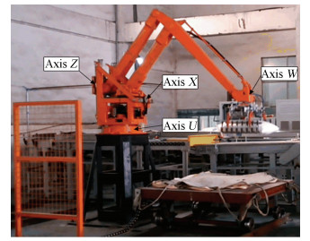
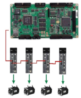
The approach has been tested on a 4-axes palletizer robot (Fig. 1), controlled by a PMAC (Program Multiple Axis Controller) device (Fig. 2), based on the Ethernet protocol. Each axis, which named U, Z, X and W, is actuated by a brush-less AC servo motor and controlled by a general model for an industrial axis PID control scheme. The gripper (the end effector) is loaded with a bag weighing nearly 50 kilos. The experiment is composed of two procedures, as follows:
|
Figure 1 The 4-axes palletizer robot for testing the approach |
|
Figure 2 The control system based on PMAC |
5.1 Minimum Time Based on Interval Analysis
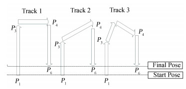
There are three common geometric tracks in the palletizing operation and they are shown in Fig. 3.
|
Figure 3 Three common geometric tracks |
Generally speaking, Track 1 is the easiest way to complete the palletize process. Meantime, it has a fatal weakness of low efficiency to handle the goods. Track 2 increases the process speed compared with Track 1, but it may collide with the obstacle due to a relative low climb height. Having avoided the above drawbacks, Track 3 has a big advantage in the processing efficiency, so it is widely used in the practical palletizing operation.
Two steps are necessary to be set up before performing the task of a whole palletizing operation:
1) A sequence of via-points in the joint space is obtained from given path in the operating space by applying inverse kinematics transformation. They are also called the input data, as reported in Table 1;
| Table 1 Via-points of each robot manipulator joint |
2) The numeric values of the kinematic constraints are determined based on the structural constraints of the manipulator, as reported in Table 2.
| Table 2 Kinematic constraints of each robot manipulator joint |
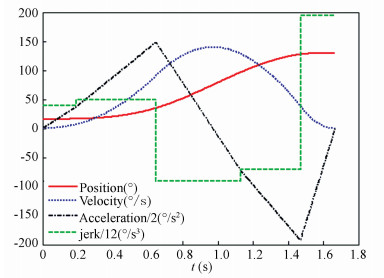
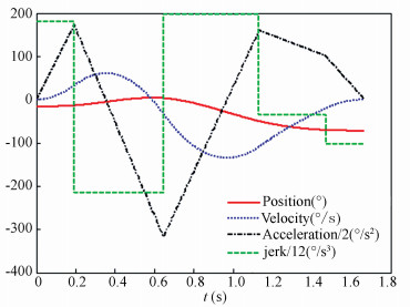
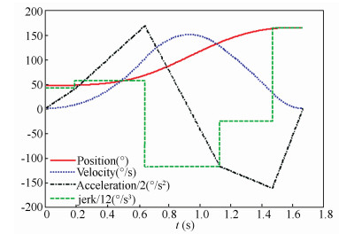
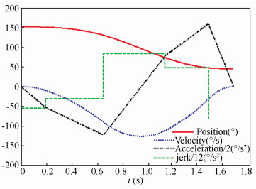
In order to conduct the test in the real manipulator, the above mentioned task has been simulated in MatLabTM software based on the proposed approach. According to the procedure in Section 3, the initial time intervals hi=0.6 s(i=1, 2, .., 5). To update hi with the new hi', each λi is decided through Eq.(7). When the difference between hi' and hi is less than 10-8, the procedure comes to an end. Figs. 4-7 show the final optimal time trajectories and their derivatives up to the third-order.
|
Figure 4 Resulting joint value: Axis U |
|
Figure 5 Resulting joint value: Axis Z |
|
Figure 6 Resulting joint value: Axis X |
|
Figure 7 |
The total execution time of the task is 1.667 5 s and 25 iterations are carried out to achieve the optimal time. The accelerations and jerks of all joints in the figures are scaled down by 2 and 12, respectively. Axis U’s results are similar to Axis X’s results because their position values are monotone increasing function of time. While Axis W’s position value is a monotone decreasing function of time. The non-monotonic position value of Axis W causes a lager acceleration during the robot movement. Compared with the values in Table 2, all the results satisfy the kinematic constraints of the robot manipulator joint. It is worth noting that, the values of each joint’s velocity and acceleration are continuous functions. Meantime, at the initial and the ending moments, the velocity and acceleration are all configured as zero and the jerk is bounded. Benefit from these features, the joint acceleration, which is in direct proportion to the needed output torque, is vital for the stability of the overall movements.
The minimumtime obtained by the global optimization techniques in Refs. [20-21] is 1.655 0 s. But the algorithms are more sophisticated and use over 50 000 iterations to achieve a better time. Though with about 0.76% time increase, the proposed approach has a clear advantage on the solution structure and computation time.
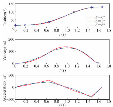
5.2 Smoothing Spline with a Prescribed Tolerance Integrating the time intervalsh=[0.191 6 s, 0.453 5 s, 0.485 5 s, 0.339 5 s, 0.197 4 s]T obtained by the first procedure into the smooth procedure, the time sequence
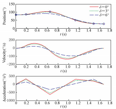
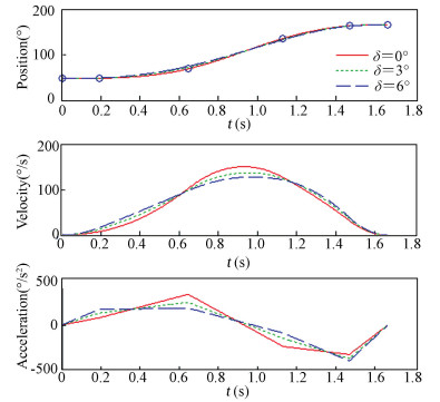
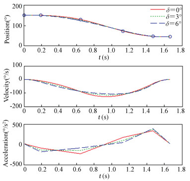
T=[0 s, 0.191 6 s, 0.645 1 s, 1.130 6 s, 1.470 1 s, 1.667 5 s]T can be determined. The virtual knots are designed to meet the joints’ initial and final conditions and their values are [16.45°, -13.89°, 47.48°, 150.34°]T and [127.49°, -70.68°, 162.89°, 47.07°]T. Then the vector q in Eq. (10) can be obtained from Table 1. W=diag{0, 1, 1, 1, 1, 0}, which means the initial and final points are the same for all kinds of trajectories. Applying the proposed smoothing technique for each axis in the simulation, notable smoother trajectories can be obtained, which are shown in Figs. 8-11.
|
Figure 8 Smoothing result: Axis U |
|
Figure 9 Smoothing result: Axis Z |
|
Figure 10 Smoothing result: Axis X |
|
Figure 11 Smoothing result: Axis W |
The solid lines in Figs. 8-11 are the trajectories without smooth process, which are in correspondence with Figs. 4-7. There are two kinds of approximate trajectories, which are represented by dotted lines and dash lines, respectively. And their approximation errors δ are 3°and 6°, respectively. It can be seen that the smaller δ is, the closer the smoothed trajectory with the initial one. By irritating the three step procedure in Section 4, the suitable value of μ can be found. The values of μ and the decrement rates of acceleration for each joint are listed in Table 3.
| Table 3 The values of μ and acceleration decrement rates for each joint |
As shown in Table 3, the larger δ can generate a smoother trajectory. By adjusting the variable δ, the trajectory can be constructed as smooth as possible. Meantime, the total execution time does not get any longer.
6 ConclusionsIn the present paper, a fast approach based on minimization of two objective function that takes into account both the execution time and the smoothness along the whole trajectory has been described. The trajectory is clamped with cubic splines and kinematic constraints on the robot motion are considered.
Unlike many other trajectory planning techniques[16-18], the proposed approach deals with the relationship between time and smooth from another perspective. Namely, the optimal time and smoothness no longer have opposite effect on the trajectory, but obtained with a two-step procedure. Compared with the algorithm proposed in Refs. [20-21], the test results have shown the effectiveness of the approach in performing the minimum-time trajectory. By adjusting the track error of the via-points with a prescribed tolerance, the trajectory has been greatly smoothed without increasing the execution time. The smooth procedure has been formulated in an analytical form, for which few iterations are enough to process. And the procedure has been validated by the experimental results.
Future work will be devoted to energy optimization, as well as to compare other trajectory forms founded in the literature.
| [1] |
Bobrow J E, Dubowsky S, Gibson J S. Time-optimal control of robotic manipulators along specified paths.
The International Journal of Robotics Research, 1985 , 4 (3) : 3-17.
DOI:10.1177/027836498500400301 ( 0) 0)
|
| [2] |
Gosselin C M, Hadj-Messaoud A. Automatic planning of smooth trajectories for pick-and-place operations.
Journal of Mechanical Design, 1993 , 115 (3) : 450-456.
DOI:10.1115/1.2919211 ( 0) 0)
|
| [3] |
Gasparetto A, Zanotto V. A new method for smooth trajectory planning of robot manipulators.
Mechanism and Machine Theory, 2007 , 42 (4) : 455-471.
DOI:10.1016/j.mechmachtheory.2006.04.002 ( 0) 0)
|
| [4] |
Shin K G, McKay N D. Minimum-time control of robotic manipulators with geometric path constraints.
IEEE Transactions on Automatic Control, 1985 , 30 (6) : 531-541.
DOI:10.1109/TAC.1985.1104009 ( 0) 0)
|
| [5] |
Balkan T. A dynamic programming approach to optimal control of robotic manipulators.
Mechanics Research Communications, 2008 , 25 (2) : 225-230.
( 0) 0)
|
| [6] |
Lo Bianco C G, Piazzi A. Minimum-time trajectory planning of mechanical manipulators under dynamic constraints.
International Journal of Control, 2002 , 75 (13) : 967-980.
DOI:10.1080/00207170210156161 ( 0) 0)
|
| [7] |
Porawagama C D, Munasinghe S R. Reduced jerk joint space trajectory planning method using 5-3-5 spline for robot manipulators. Proceedings of 7th International Conference on Information and Automation for Sustainability.Piscataway:IEEE, 2014. 1-6. doi:10.1109/ICIAFS.2014.7069580.
( 0) 0)
|
| [8] |
Boscariol P, Gasparetto A, Vidoni R. Planning continuous-jerk trajectories for industrial manipulators. ASME 2012 11th Biennial Conference on Engineering Systems Design and Analysis. American Society of Mechanical Engineers, 2012: 127-136. doi: 10.1115/ESDA2012-82103.
( 0) 0)
|
| [9] |
Costantinescu D, Croft E A. Smooth and time-optimal trajectory planning for industrial manipulators along specified paths. Journal of Robotic Systems, 2007, 17(5): 233-249. doi: 10.1002/(SICI)1097-4563(200005)17:5<233::AID-ROB1>3.0.CO; 2-Y.
( 0) 0)
|
| [10] |
Piazzi A, Visioli A. Global minimum-time trajectory planning of mechanical manipulators using interval analysis.
International Journal of Control, 1998 , 71 (4) : 631-652.
DOI:10.1080/002071798221713 ( 0) 0)
|
| [11] |
Bazaz S A, Tondu B. Minimum time on-line joint trajectory generator based on low order spline method for industrial manipulators.
Robotics and Autonomous Systems, 1999 , 29 (4) : 257-268.
DOI:10.1016/S0921-8890(99)00058-5 ( 0) 0)
|
| [12] |
Kyriakopoulos K J, Saridis G N. Minimum jerk path generation. Proceedings of 1988 IEEE International Conference on Robotics and Automation, Piscataway:IEEE, 1988.364-369.
( 0) 0)
|
| [13] |
Piazzi A, Visioli A. Global minimum-jerk trajectory planning of robot manipulators.
IEEE Transactions on Industrial Electronics, 2000 , 47 (1) : 140-149.
DOI:10.1109/41.824136 ( 0) 0)
|
| [14] |
Piazzi A, Visioli A. An interval algorithm for minimum-jerk trajectory planning of robot manipulators.
Proceedings of the 36th IEEE Conference on Decision and Control. Piscataway: IEEE, 1997 , 2 : 1924-1927.
DOI:10.1109/CDC.1997.657874 ( 0) 0)
|
| [15] |
Gasparetto A, Zanotto V. Optimal trajectory planning for industrial robots.
Advances in Engineering Software, 2010 , 41 (4) : 548-556.
DOI:10.1016/j.advengsoft.2009.11.001 ( 0) 0)
|
| [16] |
Lombai F, Szederkényi G. Throwing motion generation using nonlinear optimization on a 6-degree-of-freedom robot manipulator. IEEE International Conference on Mechatronics. Piscataway: IEEE, 2009.1-6. doi:10.1109/ICMECH.2009.4957138.
( 0) 0)
|
| [17] |
Lombai F, Szederkényi G. Trajectory tracking control of a 6 degree of freedom robot arm using nonlinear optimization. Proceedings of 10th IEEE International Workshop on Advanced Motion Control, Piscataway: IEEE, 2008.655-660. doi:10.1109/AMC.2008.4516144.
( 0) 0)
|
| [18] |
Zanotto V, Gasparetto A, Lanzutti A, et al. Experimental validation of minimum time-jerk algorithms for industrial robots.
Journal of Intelligent & Robotic Systems, 2011 , 64 (2) : 197-219.
( 0) 0)
|
| [19] |
Liu H, Lai X, Wu W. Time-optimal and jerk-continuous trajectory planning for robot manipulators with kinematic constraints.
Robotics and Computer-Integrated Manufacturing, 2013 , 29 (2) : 309-317.
DOI:10.1016/j.rcim.2012.08.002 ( 0) 0)
|
| [20] |
Gasparetto A, Zanotto V. A technique for time-jerk optimal planning of robot trajectories.
Robotics and Computer-Integrated Manufacturing, 2008 , 24 (3) : 415-426.
DOI:10.1016/j.rcim.2007.04.001 ( 0) 0)
|
| [21] |
Tangpattanakul P, Meesomboon A, Artrit P. Optimal Trajectory of Robot Manipulator Using Harmony Search Algorithms. Recent Advances In Harmony Search Algorithm. Berlin:Springer, 2010. 23-36.
( 0) 0)
|
| [22] |
Lin C S, Chang P R, Luh J Y S. Formulation and optimization of cubic polynomial joint trajectories for industrial robots.
IEEE Transactions on Automatic Control, 1983 , 28 (12) : 1066-1074.
DOI:10.1109/TAC.1983.1103181 ( 0) 0)
|
| [23] |
Biagiotti L, Melchiorri C. Trajectory Planning for Automatic Machines and Robots. Berlin:Springer Science & Business Media, 2008.
( 0) 0)
|
| [24] |
Biagiotti L, Melchiorri C. Smooth trajectories for high-performance multi-axes automatic machines.
Mechatronic Systems, 2006 , 4 (1) : 175-180.
( 0) 0)
|
 2016, Vol. 23


