2. Mechanical and Electronic Engineering Department, Heilongjiang Institute of Technology, Harbin 150050, China;
3. Materials Science & Engineering School, Beijing University of Aeronautics & Astronautics, Beijing 100194, China
Fiber-reinforced polymer matrix composite has already proven to be useful in today's aircraft industry due to their lightweight properties. These structural components, though, are often assembled using mechanically fastened joints. And mechanically fastened joints have generally been used for highly loaded composite components. But as is well known, the degradation and failure of aircraft structures frequently initiate at the joints, which poses a particularly challenging problem for engineering mechanic specialists. Therefore, the adequacy of joint design exerts strong influence on safety, durability and reliability of the construction.
In the past few years, both the theoretical analysis and the experimental research on the mechanically fastened joints of the composite laminates structure had been done. In terms of experimental research, several significant research papers on fastener joints had been published, examining the dependence on specimen geometry and layer orientation. Crews[1] reported that bolt clamp-up force exerted a significant effect on static strength and fatigue limit. Eriksson[2] had shown that bearing strength was influenced by several important parameters, including lateral constraint conditions and ply orientations. Wang et al.[3] used bearing response and bearing strength of bolted joints to examine the bearing failure mechanism as a function of clamping pressure. In recent years, many scholars also made a lot of experimental researches on the bearing strength of the bolt jointed composite structure, such as Xiao[4], Riccio[5] and Sen[6] etc. But in the past study, the effect of the test fixture on the bearing strength was not considered. The test fixture was the main device used for testing the bearing strength. In order to obtain the accurate experimental results, the effect of the test fixture on the bearing strength should be considered in research.
In terms of analytical model, the failure analysis of mechanically fastened composite joints had been performed by a method that combines continuum damage mechanics[7] with finite element analysis (FEA)[8-10]. Several analytical models had already been developed and documented in Refs.[11-15]. In these analytical models, the failure and the properties of the micro constitute material is not considered. However, the properties of the fiber reinforced resin matrix composite were closely related to its constitute properties. So the macro-micro multi-scale analytical model should be created in order to accurately predict the bearing strength and the failure damage of the bolt jointed composite laminates structure.
In this paper, the macro-micro multi-scale analytical model of the single-shear bolt jointed composite laminates structure is created. And in this model, both the test fixture and the constituted material properties including the fiber, the matrix and the interphase are considered. The rest of this paper is organized as follows: in section 2, the test on the bearing strength of the single-shear bolt jointed composite laminates structure is done and the effect of the test fixture on the experimental results is analyzed. In section 3, we present our macro-micro multi-scale numerical model for the single-shear bolt jointed composite laminates structure combining the Generalized Method of Cells based on ABAQUS software and its user subroutine USDFLD. Based on the model, the effect of the test fixture on the bearing strength of the bolt jointed composite laminates structure is analyzed further. In section 4, the important conclusions are drawn.
2 Experiment 2.1 Materials and PropertiesThe carbon fiber T700 and the bismaleimide resin (BMI) is selected respectively as the reinforced material and the matrix material of the composite laminates used in the test. Then the composite laminates are made of the prepregs T700/BMI, which are provided by AVIC Beijing Institute of Aeronautical Materials. And the mechanical properties of the constitute materials including the T700 carbon fiber and the BMI resin are listed in Table 1.
| Table 1 Mechanical properties of T700 carbon fiber and the bismaleimide (BMI) resin |
2.2 Specimen Preparation
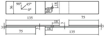
The geometric dimension of the composite laminates specimen used in the testing is shown in Fig. 1 according to the testing standard ASTM D 5961-B[16]. And as for the lamina design for the composite laminates, the followed conditions should be satisfied, such as the balanced and the symmetric stacking sequences, the certain percentage for the different layer angles and the even distribution for the same layer angle along the direction of the thickness of the composite laminates specimen. So the layup setting of the composite laminates specimen is listed in Table 2.
|
Figure 1 The geometric dimensioning of the composite laminates specimen in ASTM D5961-B |
| Table 2 Layup setting of the composite laminates specimen |
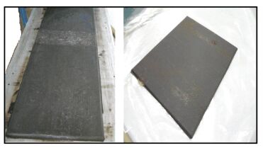
In this research, the autoclave moulding process is selected to make the composite laminates specimen. And the related technical parameters are as follows. Firstly, the autoclave is vacuumized at room temperature and the vacuum degree is not less than 0.095 MPa. Then, the 0.65-0.75 MPa pressure is added when the temperature is increased up to 100-120 ℃ at the speed of 1.5-2.0 ℃/min. The temperature is continued to increase up to 150-180 ℃ and is held on 3 h. After that, the temperature is further increased to 200±5 ℃ at the speed of 1.5-2.0 ℃/min and is kept on 4.5-5 h under the condition of keeping press. Finally, the temperature is cool down to 60 ℃ at the speed of no more than 2.5 ℃/min or it is natural cooling in the autoclave. The composite laminates are shown in Fig. 2.
|
Figure 2 Composite laminates |
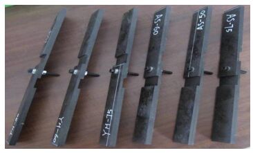
Now, according to Fig. 1, the composite laminates are cut into the required dimension by using the milling cutter. And the connection hole on the specimen is drilled by the high speed drilling machine. The single-shear bolt jointed composite laminates testing specimen is done as Fig. 3. It should be illustrated that the clamping part at the two ends of the specimen is glue jointed.
|
Figure 3 The testing specimen |
2.3 Installation of the Specimen and the Fixture
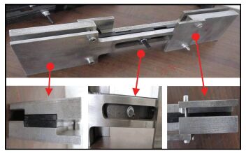
The test fixture used in the ASTM D5961-B is comparatively complex, which is composed of three main parts, that is, long grip, short grip and support plate. The test fixture is shown in Fig. 4 and its detail design and functions are introduced as follows.

|
Figure 4 The parts of the test fixture in ASTM D5961-B |
Firstly, it can be clearly seen that the open slot is cut on the long grip, which is used to facilitate the thermocouple, the fastener and the extensometer can be installed easily. Secondly, the width of the long grip is less than that of the testing specimen in order to install the extensometer on the side of the specimen. Finally, on the one end of the long grip and the short grip the ladder-like design is adopted, making the specimen be gripped better and protecting the specimen not to be damaged. And on the other end of the long grip and the short grip, the V-type groove fit is designed, making the fixture not be damaged during the process of loading.
During the process of installation, the gap between the long grip and the support plate should be nominally equal to 0 and it is not greater than 0.12 mm. If the gap is greater than 0.12 mm, the stainless steel gasket should be used to fill into the gap. Then the grade 12.9 high strength inside hexagon bolt is selected and is used as the connection bolts. And in order to avoid the slipping of the bolts, both the gasket and the spring washer are used with the bolts. The 3 N·m pre-tightening force is applied onto the bolt. In addition, it should be paid attention that the long grip should be aligned with the short grip during the process of installation. The assembled specimen and fixture is shown in Fig. 5.
|
Figure 5 The assembled specimen and test fixture |
2.4 Experiment and Results Analysis
WDW-200 electronic universal testing machines are used in the test. And the extensometer is used to measure the deformation of the specimen hole. It is worth noting that the extensometer should not be interfered with the fixture[17], as shown in Fig. 6.
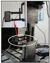
|
Figure 6 Installation for the extensometer |
Before testing, the 2 kN pre-load is applied onto the specimen firstly in order to eliminate the space between the bolt and the specimen hole and then it unloads. After that, the specimen is loaded continuously until the maximum loading decreased down to 30%. During the whole process, the loading rate of the testing machine is always maintained at 1 mm/min. The stress-stain curve of the specimen is shown in Fig. 7.

|
Figure 7 The testing results |
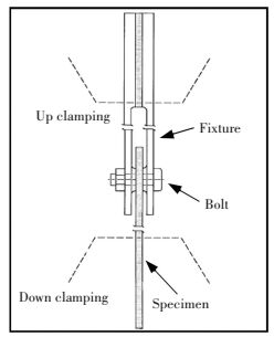
From Fig. 7, it can be seen that the repeatability of the stress-strain curve is better. But the obvious peak value on the initial phase of the curve is not appeared, which is different from the testing results of the double-shear bolt jointed composite laminates structure. (For the purpose of comparison, the test of the double-shear bolt jointed composite laminates structure made with the same material is also done based on the standard ASTM D5961-A. And its schematic diagram is shown in Fig. 8) More importantly, the main strength parameters of the single-shear bolt jointed composite laminates structure including the offset bearing strength σbr (σbr2% and σbr4%) and the limited bearing strength σbru[18] can be obtained from the above stress-stain curve and they are listed in Table 3. (The bearing strength parameters of the double-shear bolt jointed composite laminates structure are also listed in Table 3)
|
Figure 8 The schematic diagram of the double-shear bolt jointed structure |
| Table 3 The main strength indexes of the single-shear bolt jointed composite laminates structure |
From Table 3, it can be seen that all the bearing strength parameters of the single-shear bolt jointed composite laminates structure are less than that of the double-shear bolt jointed composite laminates structure. And they are lowered by 28.4%, 21.6% and 36.7% separately. From the standpoint of the testing process, the main reasons are analyzed as follows:
Firstly, the additional couple is generated during the process of single-shear connection structure testing. Under this condition, the specimen failure will be happened in advance. So the testing bearing strength of the specimen is lower.
Secondly, during the process of loading, the fastener will rotate and deform. So a part of the bolt will contact with the two sides of the specimen. This may lead to the stress concentration at this position and thus make the head of the fastener be embedded into the specimen, which is shown in Fig. 9. So the local failure will occur on the composite laminates specimen, which accelerates the crack propagation and decreases the bearing strength of the single-shear bolt jointed composite laminates structure.

|
Figure 9 The fastener embedded into the specimen after deforming |
In addition, it is worth pointing out that there is large difference by comparing the dispersion of the bearing strength of the single-shear bolt jointed composite laminates structure with that of the double-shear bolt jointed composite laminates structure. Especially for the 2% offset bearing strength σbr2%, it can be seen from Table 3 that the CV-σbr2% of the single-shear bolt jointed composite laminates structure is much larger than that of the double-shear bolt jointed composite laminates structure. From the standpoint of the testing process, the main reasons are as follows:
Firstly, the loading applied onto the specimen is transferred by the friction between the fixture and the specimen. So if the clamping force is too small, the friction force is not large enough, the skid phenomenon will occur between the fixture and the specimen. On the contrary, if the clamping force is too large, the end of the specimen will be damaged. Both the two cases will affect the testing results. Thus it can be seen that the uncertainty of clamping force applied during the process of testing is one of the reasons that result in the greater discreteness of the testing results.
Secondly, the ladder-like structure of the fixture used in the testing will result in the incomplete contaction between the specimen and the fixture during the process of the specimen installation, as shown in Fig. 10. This is another reason that results in the greater discreteness of the testing results.

|
Figure 10 The incomplete contaction between the specimen and the fixture during the testing |
3 Numerical Simulation
The macro-micro multi-scale numerical model of the single-shear bolt jointed composite laminates structure combined with the improved "Generalized Method of Cells (GMC)"[19] is created based on the software ABAQUS firstly. Then the numerical model is verified with the experimental results and it is used to characterize and analyze the effect of the test fixture on the bearing strength of the single-shear bolt jointed composite laminates structure. This may be used to instruct the testing process and also lay the foundation for the improvement and the design of the test fixture in the future research.
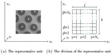
3.1 The GMC Model[20]For the fiber reinforced matrix composite, there is a certain regularity and statistical homogeneity for the distribution of the fibers in the matrix. So the representative unit cell (RVE) can be selected and be used to research the macro properties of this kind of material. The RVE is shown in Fig. 11.
|
(a) The representative unit (b) The division of the representative unit Figure 11 The representative unit cell and its division |
The local coordinate is created for the RVE and the X1 is the longitude of the fiber, and the X2, X3 is separately the transverse of the fiber. The symbol l and h are the geometric dimension of the RVE. In the local coordinate, the RVE is divided into Nβ×Nγ subcells (β=1, 2, …, Nβ, γ=1, 2, …, Nγ) and the every subcell is given the relevant material properties.
Based on the hypothesis of first-order linear displacement in the RVE, the displacement of the subcell is:
| $u_i^{\left( {\beta \gamma } \right)} = \omega _i^{\left( {\beta \gamma } \right)} + x_2^{\left( \beta \right)}\phi _i^{\left( {\beta \gamma } \right)} + x_3^{\left( \gamma \right)}\psi _i^{\left( {\beta \gamma } \right)}$ |
where subscript i=1, 2, 3 is the direction of the coordinate; the superscript (βγ) is the serial number of the subcell and the β=1, 2, …, Nβ, γ=1, 2, …, Nγ; ωi(βγ) is the displacement of the subcell center; ϕi(βγ), ψi(βγ) is the differential variables related to the subcell stain.
According to the homogenization theory, the stress and the strain of the RVE is the average value of stress and strain of the subcell in the RVE, that is:
| $\begin{array}{l} \bar \sigma = \frac{1}{{hl}}\sum\limits_{\beta = 1}^{{N_\beta }} {\sum\limits_{\gamma = 1}^{{N_\gamma }} {{h_\beta }{l_\gamma }{{\bar \sigma }^{\left( {\beta \gamma } \right)}}} } \\ \bar \varepsilon = \frac{1}{{hl}}\sum\limits_{\beta = 1}^{{N_\beta }} {\sum\limits_{\gamma = 1}^{{N_\gamma }} {{h_\beta }{l_\gamma }{{\bar \varepsilon }^{\left( {\beta \gamma } \right)}}} } \end{array}$ |
Based on the continuity hypothesis of the stress and the displacement on the interface of the subcell, the relation between the volume-averaged subcell strains and the RVE strains is:
| $\bar \varepsilon _{11}^{\left( {\beta \gamma } \right)} = {{\bar \varepsilon }_{11}},\;\;\;\beta = 1,2, \cdots ,{N_\beta };\;\;\;\gamma = 1,2, \cdots ,{N_\gamma }$ | (1) |
| $\sum\limits_{\beta = 1}^{{N_\beta }} {{h_\beta }\bar \varepsilon _{22}^{\left( {\beta \gamma } \right)}} = h{{\bar \varepsilon }_{22}},\;\;\;\gamma = 1,2, \cdots ,{N_\gamma }$ | (2) |
| $\sum\limits_{\beta = 1}^{{N_\beta }} {{h_\beta }\bar \varepsilon _{12}^{\left( {\beta \gamma } \right)}} = h{{\bar \varepsilon }_{12}},\;\;\;\gamma = 1,2, \cdots ,{N_\gamma }$ | (3) |
| $\sum\limits_{\gamma = 1}^{{N_\gamma }} {{l_\gamma }\bar \varepsilon _{33}^{\left( {\beta \gamma } \right)}} = l{{\bar \varepsilon }_{33}},\;\;\;\beta = 1,2, \cdots ,{N_\beta }$ | (4) |
| $\sum\limits_{\gamma = 1}^{{N_\gamma }} {{l_\gamma }\bar \varepsilon _{13}^{\left( {\beta \gamma } \right)}} = l{{\bar \varepsilon }_{13}},\;\;\;\beta = 1,2, \cdots ,{N_\beta }$ | (5) |
| $\sum\limits_{\beta = 1}^{{N_\beta }} {\sum\limits_{\gamma = 1}^{{N_\gamma }} {{h_\beta }{l_\gamma }\bar \varepsilon _{23}^{\left( {\beta \gamma } \right)}} } = hl{{\bar \varepsilon }_{23}}$ | (6) |
This system of equations can be written in the matrix form:
| ${\mathit{\boldsymbol{A}}_G}{{\mathit{\boldsymbol{\bar \varepsilon }}}_s} = \mathit{\boldsymbol{J}}\bar \varepsilon $ | (7) |
The matrix AG contains terms that describe the internal geometry of the subcell. The vector εs=(ε(11) , …, ε(NβNγ), ) with dimension 6NbNg contains the six volume-averaged strain components for each of the NbNg subcells. The matrix J contains the RVE dimensions.
The relation between the volume-averaged subcell stress and the RVE stress is:
| $\begin{array}{l} \bar \sigma _{22}^{\left( {1\gamma } \right)} = \bar \sigma _{22}^{\left( {2\gamma } \right)} = \cdots = \bar \sigma _{22}^{\left( {{N_\beta }\gamma } \right)} = \mathit{\boldsymbol{T}}_{22}^{\left( \gamma \right)},\gamma = 1,2, \cdots ,{N_\gamma }\\ \bar \sigma _{33}^{\left( {\beta 1} \right)} = \bar \sigma _{33}^{\left( {\beta 2} \right)} = \cdots = \bar \sigma _{33}^{\left( {\beta {N_\gamma }} \right)} = \mathit{\boldsymbol{T}}_{22}^{\left( \beta \right)},\beta = 1,2, \cdots ,{N_\beta }\\ \bar \sigma _{21}^{\left( {1\gamma } \right)} = \bar \sigma _{21}^{\left( {2\gamma } \right)} = \cdots = \bar \sigma _{21}^{\left( {{N_\beta }\gamma } \right)} = \mathit{\boldsymbol{T}}_{21}^{\left( \gamma \right)} = \mathit{\boldsymbol{T}}_{12}^{\left( \gamma \right)},\gamma = 1,\\ \;\;\;\;\;\;\;\;\;\;2, \cdots ,{N_\gamma }\\ \bar \sigma _{31}^{\left( {\beta 1} \right)} = \bar \sigma _{31}^{\left( {\beta 2} \right)} = \cdots = \bar \sigma _{31}^{\left( {\beta {N_\gamma }} \right)} = \mathit{\boldsymbol{T}}_{31}^{\left( \beta \right)} = \mathit{\boldsymbol{T}}_{13}^{\left( \beta \right)},\beta = 1,2,\\ \;\;\;\;\;\;\;\;\;\; \cdots ,{N_\beta }\\ \bar \sigma _{23}^{\left( {1\gamma } \right)} = \bar \sigma _{23}^{\left( {2\gamma } \right)} = \cdots = \bar \sigma _{23}^{\left( {{N_\beta }\gamma } \right)} = \mathit{\boldsymbol{T}}_{23}^{\left( \gamma \right)} = \bar \sigma _{32}^{\left( {\beta 1} \right)} = \bar \sigma _{32}^{\left( {\beta 2} \right)} = \\ \;\;\;\;\;\;\;\;\;\; \cdots = \bar \sigma _{32}^{\left( {\beta {N_\gamma }} \right)} = \mathit{\boldsymbol{T}}_{32}^{\left( \beta \right)} = {\mathit{\boldsymbol{T}}_{23}} \end{array}$ |
where T22γ, T21γ and T23γ is the interfacial normal stress and the shear stress for a fixed column of subcells; T33βT31β and T32β is the interfacial normal stress and the shear stress for a fixed row of subcells.
This system of equations can be written in the matrix form:
| ${\mathit{\boldsymbol{A}}_M}{{\mathit{\boldsymbol{\bar \varepsilon }}}_s} = 0$ | (8) |
where the matrix AM contains terms that describe the elastic properties of the subcells.
Combine the function (7) and the function (8) :
| $\mathit{\boldsymbol{\tilde A}}{{\mathit{\boldsymbol{\bar \varepsilon }}}_s} = \mathit{\boldsymbol{\tilde K\bar \varepsilon }}$ | (9) |
where
Then the function (9) is transformed to the function (10) :
| ${{\mathit{\boldsymbol{\bar \varepsilon }}}_s} = \mathit{\boldsymbol{\tilde A\bar \varepsilon }}$ | (10) |
where
Finally, the relation between the macro stiffness matrix of unidirectional fiber reinforced matrix composite and the properties and the volume content of the constituent material is created based on the volume-averaged hypothesis on the RVE. The equivalent macro stiffness matrix is:
| ${\mathit{\boldsymbol{C}}^ * } = \frac{1}{{hl}}\sum\limits_{\beta = 1}^{{N_\beta }} {\sum\limits_{\gamma = 1}^{{N_\gamma }} {{h_\beta }{l_\gamma }} } {\mathit{\boldsymbol{C}}^{\left( {\beta \gamma } \right)}}{\mathit{\boldsymbol{A}}^{\left( {\beta \gamma } \right)}}$ |
where C(βγ) is the stiffness of the subcell.
In the traditional GMC model, the dimension of the matrix A is [A]6Nβγ×6Nβγ. When the number of the subcell in the RVE is larger than 10×10, the solve efficiency of the traditional GMC model is decreased at high speed. So the application of the traditional GMC model is restricted. Then the improved GMC model with efficient solution efficiency is provided by Pindera and Bednarcyk[13].
In the improved GMC, the stress of the subcell is used as the unknown quantity. Firstly, according to the constitutive relation of the subcell, the principal strain of the subcell is expressed in terms of the subcell stress using the strain-stress equations.
| $\bar \varepsilon _{11}^{\left( {\beta \gamma } \right)} = \mathit{\boldsymbol{S}}_{11}^{\left( {\beta \gamma } \right)}\bar \sigma _{11}^{\left( {\beta \gamma } \right)} + \mathit{\boldsymbol{S}}_{12}^{\left( {\beta \gamma } \right)}\bar \sigma _{22}^{\left( {\beta \gamma } \right)} + \mathit{\boldsymbol{S}}_{13}^{\left( {\beta \gamma } \right)}\bar \sigma _{33}^{\left( {\beta \gamma } \right)}$ | (11) |
| $\bar \varepsilon _{22}^{\left( {\beta \gamma } \right)} = \mathit{\boldsymbol{S}}_{12}^{\left( {\beta \gamma } \right)}\bar \sigma _{11}^{\left( {\beta \gamma } \right)} + \mathit{\boldsymbol{S}}_{22}^{\left( {\beta \gamma } \right)}\bar \sigma _{22}^{\left( {\beta \gamma } \right)} + \mathit{\boldsymbol{S}}_{23}^{\left( {\beta \gamma } \right)}\bar \sigma _{33}^{\left( {\beta \gamma } \right)}$ | (12) |
| $\bar \varepsilon _{33}^{\left( {\beta \gamma } \right)} = \mathit{\boldsymbol{S}}_{13}^{\left( {\beta \gamma } \right)}\bar \sigma _{11}^{\left( {\beta \gamma } \right)} + \mathit{\boldsymbol{S}}_{23}^{\left( {\beta \gamma } \right)}\bar \sigma _{22}^{\left( {\beta \gamma } \right)} + \mathit{\boldsymbol{S}}_{33}^{\left( {\beta \gamma } \right)}\bar \sigma _{33}^{\left( {\beta \gamma } \right)}$ | (13) |
Then, the function (1) is substituted into the function (11), so the axial stress of the subcell is:
| $\bar \sigma _{11}^{\left( {\beta \gamma } \right)} = \frac{1}{{\mathit{\boldsymbol{S}}_{11}^{\left( {\beta \gamma } \right)}}}\left[ {{{\bar \varepsilon }_{11}} - \mathit{\boldsymbol{S}}_{12}^{\left( {\beta \gamma } \right)}\bar \sigma _{22}^{\left( {\beta \gamma } \right)} - \mathit{\boldsymbol{S}}_{13}^{\left( {\beta \gamma } \right)}\bar \sigma _{33}^{\left( {\beta \gamma } \right)}} \right]$ | (14) |
The function (14) is substituted into the Eqs.(12)-(13) :
| $\begin{array}{l} \bar \varepsilon _{22}^{\left( {\beta \gamma } \right)} = \frac{{\mathit{\boldsymbol{S}}_{12}^{\left( {\beta \gamma } \right)}}}{{\mathit{\boldsymbol{S}}_{11}^{\left( {\beta \gamma } \right)}}}{{\bar \varepsilon }_{11}} + \left( {\mathit{\boldsymbol{S}}_{22}^{\left( {\beta \gamma } \right)} - \frac{{{{\left( {\mathit{\boldsymbol{S}}_{12}^{\left( {\beta \gamma } \right)}} \right)}^2}}}{{\mathit{\boldsymbol{S}}_{11}^{\left( {\beta \gamma } \right)}}}} \right)\bar \sigma _{22}^{\left( {\beta \gamma } \right)} + \\ \;\;\;\;\;\;\;\;\;\;\left( {\mathit{\boldsymbol{S}}_{23}^{\left( {\beta \gamma } \right)} - \frac{{\mathit{\boldsymbol{S}}_{12}^{\left( {\beta \gamma } \right)}\mathit{\boldsymbol{S}}_{13}^{\left( {\beta \gamma } \right)}}}{{\mathit{\boldsymbol{S}}_{11}^{\left( {\beta \gamma } \right)}}}} \right)\bar \sigma _{33}^{\left( {\beta \gamma } \right)} \end{array}$ | (15) |
| $\begin{array}{l} \bar \varepsilon _{33}^{\left( {\beta \gamma } \right)} = \frac{{\mathit{\boldsymbol{S}}_{12}^{\left( {\beta \gamma } \right)}}}{{\mathit{\boldsymbol{S}}_{11}^{\left( {\beta \gamma } \right)}}}{{\bar \varepsilon }_{11}} + \left( {\mathit{\boldsymbol{S}}_{23}^{\left( {\beta \gamma } \right)} - \frac{{\mathit{\boldsymbol{S}}_{12}^{\left( {\beta \gamma } \right)}\mathit{\boldsymbol{S}}_{13}^{\left( {\beta \gamma } \right)}}}{{\mathit{\boldsymbol{S}}_{11}^{\left( {\beta \gamma } \right)}}}} \right)\bar \sigma _{22}^{\left( {\beta \gamma } \right)} + \\ \;\;\;\;\;\;\;\;\;\;\left( {\mathit{\boldsymbol{S}}_{33}^{\left( {\beta \gamma } \right)} - \frac{{{{\left( {\mathit{\boldsymbol{S}}_{13}^{\left( {\beta \gamma } \right)}} \right)}^2}}}{{\mathit{\boldsymbol{S}}_{11}^{\left( {\beta \gamma } \right)}}}} \right)\bar \sigma _{33}^{\left( {\beta \gamma } \right)} \end{array}$ | (16) |
Combining the stress continuity condition and substituting the Eqs.(15)-(16) into the Eqs.(2)-(3) the improved interfacial displacement continuity condition is:
| $\begin{array}{l} \sum\limits_{\beta = 1}^{\beta = {N_\beta }} {{h_\beta }\left[ {\frac{{\mathit{\boldsymbol{S}}_{12}^{\left( {\beta \gamma } \right)}}}{{\mathit{\boldsymbol{S}}_{11}^{\left( {\beta \gamma } \right)}}}{{\bar \varepsilon }_{11}} + \left( {\mathit{\boldsymbol{S}}_{22}^{\left( {\beta \gamma } \right)} - \frac{{{{\left( {\mathit{\boldsymbol{S}}_{12}^{\left( {\beta \gamma } \right)}} \right)}^2}}}{{\mathit{\boldsymbol{S}}_{11}^{\left( {\beta \gamma } \right)}}}} \right){T_{22}} + } \right.} \\ \;\;\;\;\;\left. {\left( {\mathit{\boldsymbol{S}}_{23}^{\left( {\beta \gamma } \right)} - \frac{{\mathit{\boldsymbol{S}}_{12}^{\left( {\beta \gamma } \right)}\mathit{\boldsymbol{S}}_{13}^{\left( {\beta \gamma } \right)}}}{{\mathit{\boldsymbol{S}}_{11}^{\left( {\beta \gamma } \right)}}}} \right){\mathit{\boldsymbol{T}}_{33}}} \right] = h{{\bar \varepsilon }_{22}}\\ \sum\limits_{\gamma = 1}^{\gamma = {N_\gamma }} {{l_\gamma }\left[ {\frac{{\mathit{\boldsymbol{S}}_{13}^{\left( {\beta \gamma } \right)}}}{{\mathit{\boldsymbol{S}}_{11}^{\left( {\beta \gamma } \right)}}}{{\bar \varepsilon }_{11}} + \left( {\mathit{\boldsymbol{S}}_{23}^{\left( {\beta \gamma } \right)} - \frac{{\mathit{\boldsymbol{S}}_{12}^{\left( {\beta \gamma } \right)}\mathit{\boldsymbol{S}}_{13}^{\left( {\beta \gamma } \right)}}}{{\mathit{\boldsymbol{S}}_{11}^{\left( {\beta \gamma } \right)}}}} \right){T_{22}} + } \right.} \\ \;\;\;\;\;\left. {\left( {\mathit{\boldsymbol{S}}_{33}^{\left( {\beta \gamma } \right)} - \frac{{{{\left( {\mathit{\boldsymbol{S}}_{13}^{\left( {\beta \gamma } \right)}} \right)}^2}}}{{\mathit{\boldsymbol{S}}_{11}^{\left( {\beta \gamma } \right)}}}} \right){\mathit{\boldsymbol{T}}_{33}}} \right] = l{{\bar \varepsilon }_{33}} \end{array}$ |
In the form of matrix, the functions are expressed as follows:
| $\left[ {\begin{array}{*{20}{c}} \mathit{\boldsymbol{A}} & \mathit{\boldsymbol{B}}\\ {\mathit{\boldsymbol{B'}}} & D \end{array}} \right]\left[ {\begin{array}{*{20}{c}} {{\mathit{\boldsymbol{T}}_2}}\\ {{\mathit{\boldsymbol{T}}_3}} \end{array}} \right] = \left\{ {\begin{array}{*{20}{c}} c\\ e \end{array}} \right\}{{\bar \varepsilon }_{11}} + \left\{ {\begin{array}{*{20}{c}} \mathit{\boldsymbol{H}}\\ 0 \end{array}} \right\}{{\bar \varepsilon }_{22}} + \left\{ {\begin{array}{*{20}{c}} 0\\ \mathit{\boldsymbol{L}} \end{array}} \right\}{{\bar \varepsilon }_{33}}$ | (17) |
where A, B, B′, D is the matrix of [A]Nγ×Nγ, [B]Nγ×Nβ, [B′]Nβ×Nγ, [D]Nβ×Nβ. T2=[T22(1) , …, T22(Nγ)], T3=[T33(1) , …, T33(Nβ)], [c]1×Nβ, [e]1×Nγ is the column vector contains terms that describe the geometry dimension and the flexibility parameters of the subcell. H=[h, …, h]NγT×1, L=[l, …, l]NβT×1.
By function (17), the transverse stress of the subcell σ22(βγ) and σ33(βγ) can be solved. And combined with the function (14), the axial stress of the subcell σ11(βγ) is also solved.
In the same way, the relation between the shear stress and the shear strain is:
| $\begin{array}{l} \frac{1}{2}\left( {\sum\limits_{\beta = 1}^{{N_\beta }} {{h_\beta }S_{66}^{\left( {\beta \gamma } \right)}} } \right)\mathit{\boldsymbol{T}}_{12}^{\left( \gamma \right)} = h{{\bar \varepsilon }_{12}}\\ \frac{1}{2}\left( {\sum\limits_{\gamma = 1}^{{N_\gamma }} {{l_\gamma }S_{55}^{\left( {\beta \gamma } \right)}} } \right)\mathit{\boldsymbol{T}}_{13}^{\left( \beta \right)} = l{{\bar \varepsilon }_{13}}\\ \frac{1}{2}\left( {\sum\limits_{\beta = 1}^{{N_\beta }} {\sum\limits_{\gamma = 1}^{{N_\gamma }} {{h_\beta }{l_\gamma }S_{44}^{\left( {\beta \gamma } \right)}} } } \right){\mathit{\boldsymbol{T}}_{23}} = hl{{\bar \varepsilon }_{23}} \end{array}$ |
Finally, the relation between the stress of the subcell and the macro stress of the RVE is:
| $\bar \sigma = \frac{1}{{hl}}\sum\limits_{\beta = 1}^{{N_\beta }} {\sum\limits_{\gamma = 1}^{{N_\gamma }} {{h_\beta }{l_\gamma }{{\bar \sigma }^{\left( {\beta \gamma } \right)}}} } $ | (18) |
The function (18) can be used to analyze the mesoscopic mechanical properties of the multi-phase composite.
3.2 The Macro-micro Multi-scale MethodOne of the objectives of the present work is to create a practical tool for conducting the macro-micro multi-scale progressive damage analysis and the strength prediction of the single-shear bolt jointed composite laminates structure by implementing the improved GMC model into the commercial FEM code ABAQUS. Thereby, the improved GMC model is combined with the failure criterion of the constituent material and the decay law of the constituent material properties firstly. Then it is introduced into the numerical model of the single-shear bolt jointed composite laminates structure by the port of user subroutine (USDFLD) provided by the software ABAQUS[21].
Failure criterion of the mesoscopic constituent material including the matrix failure criterion, the fiber failure criterion and the interphase failure criterion[22], they are as follows:
The matrix tension (compression) failure criterion is:
| $\begin{array}{l} {e_m} = {\left( {\frac{{{\sigma _2}}}{{{\mathit{\boldsymbol{Y}}_t}}}} \right)^2} + {\left( {\frac{{{\tau _{12}}}}{\mathit{\boldsymbol{S}}}} \right)^2},{\sigma _2} \ge 0\\ {e_m} = {\left( {\frac{{{\sigma _2}}}{{{\mathit{\boldsymbol{Y}}_c}}}} \right)^2} + {\left( {\frac{{{\tau _{12}}}}{\mathit{\boldsymbol{S}}}} \right)^2},{\sigma _2} < 0 \end{array}$ |
The fiber tensile failure criterion is:
| ${e_f} = {\left( {{\sigma _1}/{\mathit{\boldsymbol{X}}_t}} \right)^2},{\sigma _1} \ge 0$ |
where the parameter Xt is the tension strength of the fiber material, and Yt, Yc, S is the tension strength, the compression strength and the shear strength of the matrix material separately.
The interphase failure criterion is:
| ${\left( {\frac{{\left\langle {{t_n}} \right\rangle }}{{{\mathit{\boldsymbol{Y}}_n}}}} \right)^2} + {\left( {\frac{{{t_t}}}{{{\mathit{\boldsymbol{Y}}_t}}}} \right)^2} + {\left( {\frac{{{t_l}}}{{{\mathit{\boldsymbol{Y}}_l}}}} \right)^2} = 1$ |
where the symbol 〈〉 represents the returned value when the parameter tn>0. If tn < 0, the returned value is zero. The parameters Yn, Yt, Yl are the strength of the interphase along the three orthotropic directions[23].
When the above anyone failure criterion is satisfied, it is considered that the corresponding damage modes will appear. Then the properties of the constitute material begin to decay according to the corresponding decay law. Generally, two kind of decay modes, that is, the complete decay mode and the partial decay mode can be adopted in the application[24]. In this research, the former is used. So, when a certain layer of the composite laminates is damaged, this layer will lose their bearing capacity on some directions, but on the other directions, that is not. The corresponding relationship between the damage mode and the properties decay[25-26]is listed in Table 4.
| Table 4 The corresponding relationship between the damage mode and the properties decay |
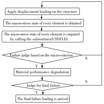
Now, the macro-micro multi-scale numerical model combined with the improved GMC method for the progressive damage analysis and the strength forecast of the single-shear bolt jointed composite laminates structure can be created based on the software ABAQUS and its user subroutine USDFLD. And the flow chart is shown in Fig. 12.
|
Figure 12 Flow chart of macro-micro multi-scale analysis combined with the improved GMC model |
3.3 The Numerical Model
Based on the software ABAQUS, the geometry model of the single-shear bolt jointed composite laminates structure is created firstly according to the ASTM D 5961-B standard and it is shown in Fig. 13. In the geometry model, it can be seen that almost all parts in the assembly are partitioned in order to mesh conveniently. And the composite laminates part is layered to[45°/0°/-45°/90°]4s according to the layer setting listed in Table 2.

|
Figure 13 The geometric model of the single-shear bolt jointed composite laminates structure |
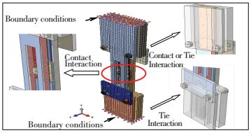
Then, the geometry model is partitioned with the suitable element. The composite laminates is constructed using eight-node continuous shell elements (SC8R) and the bolt and the fixture is constructed using the eight-node hexahedral elements (C3D8I). Fig. 14 displays a summary of the finite element meshes, the corresponding boundary conditions and the interaction relation.
|
Figure 14 The numerical model of the single-shear bolted joint composite laminates structure |
In order to make the interaction relation set up steadily among the parts and to avoid the parts rigidly move, the multi-steps are set in the analysis. It is presented as follows:
Step 1 In the initial step, the ends of the two composite laminates specimen and the ends of the fixture are all fixed.
Step 2 In the first step, the small pretension force (10 N) is applied onto the bolt. (The loading surface is cut on the bolt rod in order to apply the bolt pretension force)
Step 3 In the second step, the real pretension force 2500 N is applied onto the bolt.
Step 4 In the third step, the constraint applied onto the upper end of the single-shear bolt jointed composite laminates structure is removed but the pretension force applied on the bolt is kept unchanged.
Step 5 In the fourth step, remove the pretension force applied onto the bolt and keep the bolt at the present length. At the same time, the small displacement load (0.1 mm) is applied onto the upper end of the jointed structure. So the contact relation between the specimen and the bolt can be created steadily.
Step 6 In the final step, the whole displacement load is applied onto the jointed structure and the bearing properties of the single-shear bolt jointed composite laminates structure is analyzed.
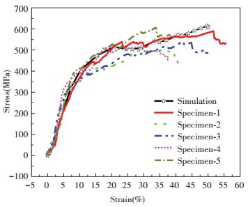
3.4 Numerical Results and DiscussionNow, the numerical model is used to analyze the bearing strength and the damage mode of the single-shear bolt jointed composite laminates structure. Fig. 15 displays the comparison between the simulated and the experimental stress-strain curve. And the macro damage pattern of the bolt jointed composite laminates is also predicted and is compared with the experimentally testing results, which is shown in Fig. 16. In addition, it is important that the distribution of the failure constitute material in different layer is predicted by the numerical model and is compared with the testing results, which is shown in Fig. 17.
|
Figure 15 The comparison between the simulated and experimentally determined stress-strain curve |

|
Figure 16 The comparison between the simulated and experimentally determined macro damage pattern |

|
Figure 17 The comparison between the simulated and experimentally determined micro constitute material damage |
From Figs. 15-17, it can be seen that the predicted results including the macro stress-strain curve, the macro damage pattern and the micro constitute material failure are all consistent with the experimental testing results. It is manifest that the created numerical model is fundamentally accurate. So it can be used to the following characterization and analysis.
3.5 The Application of the ModelIn this part, from the perspective of test fixture, the numerical model will be used to analyze the effect of the test fixture on the bearing strength of the single-shear bolt jointed composite laminates structure. Aiming at the experimental testing results and the problems discovered during the process of testing, the constrain condition, the boundary condition, the loading condition and the fixture rigid in the numerical model are changed accordingly in the following characterization and analysis.
Because of the fixture instability in the testing, the fixture and the specimen incompletely contact during the process of the specimen installation (as shown in Fig. 10). So, the effect of the incomplete contaction between the fixture and the specimen on the bearing strength is done firstly by changing the constraint conditions in the numerical model from the complete contaction state to the incomplete contaction state. The analysis results are shown in Fig. 18.

|
Figure 18 The numerical analysis for the effect of incomplete contaction on the bearing strength |
From Fig. 18, it can be seen that if the lateral of the specimen is not constrained completely during the testing, the stiffness of the single-shear bolt jointed structure will not be affected, but both of its offset bearing strength and the limited bearing strength decrease. So, during the process of specimen installation, it deserves attention that the incomplete contaction should be avoided.
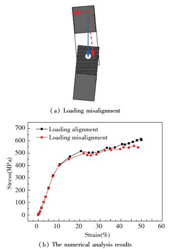
Because the constrain along the transverse direction of the specimen is not enough, the following status (as shown in Fig. 19) will appear during the process of the specimen installation. In this case, not only the Y directional loading is applied onto the specimen, but also the X directional loading is applied onto the specimen, which is shown in Fig. 19(a). So in the numerical mode, the loading is setting along the two directions to analyze its effect on the bearing strength of the single-shear bolt jointed composite laminates structure. The analysis results are shown in Fig. 19(b).
|
Figure 19 Schematic diagram of loading misalignment and the numerical analysis for the effect on the bearing strength |
From Fig. 19(b), it can be seen that if the loading applied onto the specimen is misalignment along the Y direction during the testing, although the stiffness of the single-shear bolt jointed composite structure will not be affect, its offset bearing strength and the limited bearing strength are reduced. So this case should be also avoided in the testing.
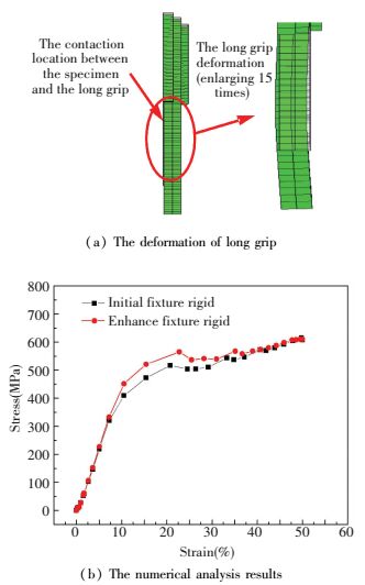
It is known that the long grip fixture (Fig. 4(a)) has two functions in the testing. The ladder-like part is used to clamp the specimen. And the open slot part is used to constrain the lateral deformation of the specimen. During the process of loading, by the contaction between the specimen and the open slot part of the long grip, the long grip will be deformed, which is shown in Fig. 20(a). So, the effect of the rigid of the long grip on the bearing strength of the single-shear bolt jointed composite laminates structure is characterized. The analysis results are shown in Fig. 20(b).
|
Figure 20 The deformation of long grip and the numerical analysis for the effect on the bearing strength |
It can be seen from Fig. 20(b) that both the rigid and the offset bearing strength of the single-shear bolt jointed composite laminates structure will be improved by enhancing the lateral rigid of the long grip. So in the testing, the rigid of the grip must be ensured in order to obtain the accurate testing results.
4 ConclusionsIn this research, the effect of the test fixture on the bearing strength of the single-shear bolt jointed composite laminates structure is analyzed based on the testing and numerical simulation. The conclusions are as follows:
1) The bearing strength of the single-shear bolt jointed composite laminates structure is lower than that of the double-shear bolt jointed composite laminates structure. The main reason is that the structure difference between the two jointed structures. And the dispersion of the testing results is rather large. It is the results of the testing fixture and the loading method used in the single-shear bolt jointed structure.
2) The macro-micro multi-scale analytical model of the single-shear bolt jointed composite laminates structure is created in this paper. And the predicted results of the model agree with the experimental results. It can be used to characterize and analyze the effect of the fixture on the testing results. And this method can be also used in the future research.
3) The numerical analysis results manifest that the incomplete clamp for the specimen, the loading misalignment and the lower rigid of the fixture will affect the testing results, that is, the testing results is lower than its true value. So these reasons should be avoided in the testing. And this research results can be used to instruct the improvement of the fixture in the future research.
| [1] |
Jr. Crews J H. Bolt-bearing fatigue of a graphite/epoxy laminate.
Presented at the ASTM Specialist Symposium on Joining of Composite Materials, Minneapolis, 1981: 131-144.
( 0) 0)
|
| [2] |
Eriksson I. On the bearing strength of bolted graphite/epoxy laminates.
Journal of Composite Materials, 1990, 24(12): 1264-1269.
( 0) 0)
|
| [3] |
Wang H S, Hung C L, Chang F K. Bearing failure of bolted composite joints. Part Ⅰ: experiments.
Journal of Composite Materials, 1996, 30(12): 1284-1313.
DOI:10.1177/002199839603001201 ( 0) 0)
|
| [4] |
Xiao Y, Ishikawa T. Bearing strength and failurebehavior of bolted composite joints (Part Ⅰ: experimental investigation).
Composites Science and Technology, 2005, 65(7/8): 1022-1031.
DOI:10.1016/j.compscitech.2005.02.011 ( 0) 0)
|
| [5] |
Riccio A, Marciano L. Effects of geometrical and material features on damage onset and propagation in single-lap bolted composite joints under tensile load: Part Ⅰ-experimental studies.
Journal of Composite Materials, 2005, 39(23): 2071-2090.
DOI:10.1177/0021998305052026 ( 0) 0)
|
| [6] |
Sen F, Pakdi M, Sayman O, et al. Experimental failure analysis of mechanically fastened joints with clearance in composite laminates under perload.
Materials & Design, 2008, 29(6): 1159-1169.
DOI:10.1016/j.matdes.2007.05.009 ( 0) 0)
|
| [7] |
Chaboche J L. Continuum damage mechanics: part I-general concepts; part Ⅱ-damage growth, crack initiation and crack growth.
Journal of Applied Mechanics, 1988, 55(1): 59-72.
DOI:10.1115/1.3173661 ( 0) 0)
|
| [8] |
McCarthy C T, McCarthy M A, Lawlor V P. Progressive damage analysis of multi-bolt composite joints with variable bolt-hole clearances.
Composites Part B: Engineering, 2005, 36(4): 290-305.
DOI:10.1016/j.compositesb.2004.11.003 ( 0) 0)
|
| [9] |
Kapti S, Sayman O, Ozen M, et al. Experimental and numerical failure analysis of carbon/epoxy laminated composite joints under different conditions.
Materials & Design, 2010, 31(10): 4933-4942.
DOI:10.1016/j.matdes.2010.05.018 ( 0) 0)
|
| [10] |
Egan B, McCarthy C T, McCarthy M A, et al. Stress analysis of single-bolt, single-lap countersunk composite joints with variable bolt-hole clearance.
Composite Structures, 2012, 94(3): 1038-1051.
DOI:10.1016/j.compstruct.2011.10.004 ( 0) 0)
|
| [11] |
Chang F K, Chang K Y. Post-failure analysis of bolted composite joints in tension or shear-out mode failure.
Journal of Composite Materials, 1987, 21(9): 809-833.
DOI:10.1177/002199838702100903 ( 0) 0)
|
| [12] |
Lessard L B, Shokrieh M M. Two-dimensional modeling of composite pinned-joint failure.
Journal of Composite Materials, 1995, 29(5): 671-97.
DOI:10.1177/002199839502900507 ( 0) 0)
|
| [13] |
Hung C L, Chang F K. Bearing failure of bolted composite joints. Part Ⅱ: model and verification.
Journal of Composite Materials, 1996, 30: 1359-1400.
DOI:10.1177/002199839603001204 ( 0) 0)
|
| [14] |
Kim S J, Hwang J S, Kim J H. Progressive failure analysis of pin-loaded laminated composites using penalty finite element method.
AIAA J, 1998, 36(1): 75-80.
DOI:10.2514/2.354 ( 0) 0)
|
| [15] |
Camanho P P, Matthews F L. A progressive damage model for mechanically fastened joints in composite laminates.
Journal of Composite Materials, 1999, 33(24): 2248-2280.
DOI:10.1177/002199839903302402 ( 0) 0)
|
| [16] |
American Society of Testing Materials. ASTM D 5961-A Standard Test Method for Bearing Response of Polymer Matrix Composite Laminates. American Society for Testing and Materials Association International. 2005.
( 0) 0)
|
| [17] |
N/A. Military Handbook-MIL-HDBK-17-1F: Composite Materials Handbook. Vol. 1. Polymer-matrix Composites Guidelines for Characterization of Structural Materials. Department of Defense, 2002.
( 0) 0)
|
| [18] |
Yi Xiao, Takashi Ishikawa. Bearing strength and failure behavior of bolted composite joints part I: Experimental investigation.
Composites Science and Technology, 2005, 65(7): 1022-1031.
DOI:10.1016/j.compscitech.2005.02.011 ( 0) 0)
|
| [19] |
Paley M, Aboudi J. Micromechanical analysis of composites by the generalized cells model.
Mechanics of Materials, 1992, 14(29): 127-139.
( 0) 0)
|
| [20] |
Pindera M J, Bednarcyk B A. An effcient implementation of the generalized method of cells for unidirectional, multi-phased composites with complex microstructures.
Composites Part B, 1999, 30(1): 87-105.
DOI:10.1016/S1359-8368(98)00040-7 ( 0) 0)
|
| [21] |
Hibbit, Karlson & Sorensen, Inc. User subroutine to define a material's mechanical behavior; 1. 1. 43: User subroutine to redefine field variables at a material point. ABAQUS User Subroutines Reference Manual. Ver. 6. 8.
( 0) 0)
|
| [22] |
Tang Zhanwen. Comparison of Strength Analysis of Composites Based on GMC and FVDAM. Harbin: Harbin Institute of Technology, 2013 (in Chinese).
( 0) 0)
|
| [23] |
Kermanidis T, Labeas G, Tserpes K I, et al. Finite element modeling of damage accumulation in bolted composite joints under incremental tensile loading. In: European Congress on Computational Methods in Applied Sciences and Engineering, Barcelona, 2000.
( 0) 0)
|
| [24] |
Tsai S W. Composites Design. Shenyang: Ministry of Aviation Industry 601Research Institution, 1988. 155-156.
( 0) 0)
|
| [25] |
Li Weizhan. Progressive Damage Analysis of Composite Laminates. Harbin: Harbin Engineering University, 2012 (in Chinese).
( 0) 0)
|
| [26] |
Okutan Baba B. Behavior of pin-loaded laminated composites.
Experimental Mechanics, 2006, 46(5): 589-600.
DOI:10.1007/s11340-006-8735-z ( 0) 0)
|
 2017, Vol. 24


