2. College of Automation Engineering, Nanjing University of Aeronautics and Astronautics, Nanjing 210016, China
Quad-rotor aircrafts have been an issue of increasing concern in recent year. The unmatched qualities of unmanned aerial vehicles (UAVs) make them have a competitive advantage in circumstances where tasks are high to pilots or operation environment is dangerous to human[1-2]. The dynamical model of a Quad-rotor aircraft is nonlinear, but also under actuated for the aircraft has only four inputs generated by four actuators that are less than the six degrees of freedom. Aircrafts are always subjected to lots of effects, such as ground effect, and friction, etc.[3-4].Because of these characteristics and effects, an ideal controller for Quad-rotor aircrafts seems to be a big challenge.
In control system, the inverse model control (IMC) scheme becomes popular for the ability to resist the disturbance and the good robustness[5]. In practice, almost every control system is nonlinear and the nonlinear characteristic is more obvious when the system operates in a wide range[6-7]. Hence, various IMC controllers have been proposed. And the process model determination plays an important role. To design a control scheme to overcome uncertainties, a black-box identification technology combined with the neural networks (NNS) has become a popular option[8]. NNS are able to approximate any nonlinear dynamic systems for any given precision[9-10]. However, most neural networks need to be trained with lots of time and often suffer from the problem of local minima and over-fitting. Moreover, there is no theoretical guidance to build an appropriate neural network in the number of hidden layers and neurons.
Support vector regression (SVR) is regarded substitutable for NNS in many areas such as regression estimation. The SVR model turns the original problem into a problem of quadratic programming (QP)which can be figured out according to QP solver[11-12]. Thus, the regression estimation can be solved by SVR to overcome the problem of local minima. In addition, the design parameters for the SVR is often easy to be tuned due to the fixed construction of SVR[13].
However, a SVR contains a large number of support vectors (SVs), so the model becomes complex correspondingly[14]. A SVR based on TS-type Fuzzy System (TS-fuzzy SVR) with a new kernel named TS-kernel is proposed in this paper. TS-fuzzy SVR combines the advantages of both fuzzy neural network and SVR. One is that the number of parameters of FNN is smaller than that of SVR generally[15]. Also SVR has high generalization ability.
This paper designed an inverse model control scheme in the attitude system of Quad-rotor aircraft using the TS-fuzzy SVR. The function of TS-fuzzy SVR is combined with TS-type kernel, in which the weight parameters and kernels are trained by SVR and clustering respectively[16-17]. Considering the size of TS-fuzzy SVR is determined only by the number of clusters, the size of network can be reduced[18]. TS-fuzzy SVR weighting parameters are based on linear SVR, and designed to endow the network with an ability of high generalization and robust function. Simulations of function approximation will verify TS-fuzzy SVR performance[19]. Although the solution possesses the global property, there exist uncertainties and disturbances which may not be trained. In order to handle the unexpected nonlinear characteristics, a new controller combined with TS-fuzzy SVR inverse model controller and PID controller is designed in the attitude system of Quad-rotor aircraft.
2 TS-fuzzy SVR Model and Training 2.1 Basic SVR ConceptsIn ε-SVR regression estimation, the aim is to seek out a function f(X) which has been up to ε deviation from the obtained targets yi for training data sets. The decision function is:
| $ \mathit{\boldsymbol{f}}\left( \mathit{\boldsymbol{X}} \right) = {\mathit{\boldsymbol{\omega }}^{\rm{T}}}\mathit{\boldsymbol{X}} + b $ | (1) |
where ω∈Rn denotes the weighted vector and b is a constant term.
The training data sets are
| $ \mathit{\boldsymbol{S}} = \left\{ {\left( {{x_1},{y_1}} \right),\left( {{x_2},{y_2}} \right), \cdots ,\left( {{x_n},{y_n}} \right)} \right\} $ | (2) |
where xi∈Rd, yi∈{-1, 1}, i=1, 2, ..., n.
Constrains are given for the training data to find a separable hyperplane with the largest margin. However, input data are often inseparable. For such case, two positive variables ξi and ξi* are introduced:
| $ \left\{ \begin{array}{l} {\mathit{\boldsymbol{\omega }}^{\rm{T}}}\mathit{\boldsymbol{X}} + b \ge {y_i} - \varepsilon - {\xi _i}\\ {\mathit{\boldsymbol{\omega }}^{\rm{T}}}\mathit{\boldsymbol{X}} + b \le {y_i} + \varepsilon + \xi _i^ * \end{array} \right. $ | (3) |
where ε is the upper boundary of the tolerance of error, ξi, ξi*≥0, i=1, 2, ..., n.
To maximize the margin between the two hyperplanes, which is 2/║ω║. Defining the Lagrangian function 2/||ω|| with Lagrange multipliers ai, βi, ai* and βi* as follows:
| $ \begin{array}{l} L\left( {\omega ,b,{a_i},a_i^ * ,{\xi _i},\xi _i^ * } \right) = \frac{1}{2}{\left\| \mathit{\boldsymbol{\omega }} \right\|^2} + C\sum\limits_{i = 1}^n {\left( {{\xi _i} + } \right.} \\ \;\;\;\;\;\;\;\;\;\;\;\;\left. {\xi _i^ * } \right) - \sum\limits_{i = 1}^n {a_i^ * \left( {{\mathit{\boldsymbol{\omega }}^{\rm{T}}}\mathit{\boldsymbol{X}} + b - {y_i} + \varepsilon + {\xi _i}} \right)} - \\ \;\;\;\;\;\;\;\;\;\;\;\;\sum\limits_{i = 1}^n {a_i^ * \left( { - {\mathit{\boldsymbol{\omega }}^{\rm{T}}}\mathit{\boldsymbol{X}} - b + {y_i} + \varepsilon + \xi _i^ * } \right)} - \\ \;\;\;\;\;\;\;\;\;\;\;\;\sum\limits_{i = 1}^n {\left( {{\beta _i}{\xi _i} + \beta _i^ * \xi _i^ * } \right)} \end{array} $ | (4) |
The gradient of L(ω, b, ai, ai*, ξi, ξi*) with respect to ω, b, βi, βi* is
| $ \left\{ \begin{array}{l} \frac{{\partial L}}{{\partial \omega }} = 0 \Rightarrow \omega = \sum\limits_{i = 1}^n {\left( {{a_i} - a_i^ * } \right){x_i}} \\ \frac{{\partial L}}{{\partial b}} = 0 \Rightarrow \sum\limits_{i = 1}^n {\left( {{a_i} - a_i^ * } \right)} = 0\\ \frac{{\partial L}}{{\partial {\xi _i}}} = 0 \Rightarrow {\beta _i} = C - {a_i}\\ \frac{{\partial L}}{{\partial \xi _i^ * }} = 0 \Rightarrow \beta _i^ * = C - a_i^ * \end{array} \right. $ | (5) |
Then the decision function becomes:
| $ f\left( x \right) = \sum\limits_{i = 1}^n {\left( {{a_i} - a_i^ * } \right){x_i} \cdot x + b} $ | (6) |
The kernel function maps the input into output F through a nonlinear function φ(·):x→F while the hyperplanes are nonlinear. The kernel function is given as follows:
| $ K\left( {\mathit{\boldsymbol{X}},\mathit{\boldsymbol{Z}}} \right) = \left\langle {\varphi \left( \mathit{\boldsymbol{X}} \right),\varphi \left( \mathit{\boldsymbol{Z}} \right)} \right\rangle $ | (7) |
So the decision function will be:
| $ f\left( x \right) = \sum\limits_{i = 1}^n {\left( {{a_i} - a_i^ * } \right)K\left( {{x_i},x} \right) + b} $ | (8) |
In this paper, a TS-type kernel is proposed and it is adopted as the basic function in TS-fuzzy SVR.
The model of TS-fuzzy SVR is given below:
| $ y\left( x \right) = \sum\limits_{j = 1}^k {{\omega _j}{K_{TS}}\left( {x,{d_j}} \right) + b} $ | (9) |
where k denotes the number of TS-kernels and the TS-kernels KTS(x, dj) is:
| $ {K_{TS}}\left( {x,{d_j}} \right) = \left( {x,{d_j}} \right) \cdot \exp \left\{ {\frac{{{{\left\| {x - {d_j}} \right\|}^2}}}{{\sigma _j^2}}} \right\} $ | (10) |
where dj and σj refer to the center and width of the fuzzy set respectively. And the TS-kernel can be decomposed into two single kernels:
| $ {k_{TS}}\left( {x,{x_j}} \right) = {K_1}\left( {x,{x_j}} \right) \cdot {K_2}\left( {x,{x_j}} \right) $ | (11) |
where K1(x, xj)=(x·xj) is a linear kernel, K2(x, xj)·
A TS-type fuzzy system has the following composing rule form:
Rule j: if x1 is A1j and … xm is Amj, then
| $ {y^j} = b_1^j{x_1} + \cdots + b_m^j{x_m} = \sum\limits_{i = 1}^m {b_i^j{x_i}} $ |
where xi is the jth input variable; Aij is a fuzzy set; bij is the system parameters and yj is the ith output of Rule j. And the membership degree of Aij will be:
| $ M_i^j = \exp \left\{ { - \left( {\frac{{\left( {{x_i} - d_i^j} \right)}}{{\sigma _j^2}}} \right)} \right\} $ | (12) |
The membership degree of Mij to Rule j is:
| $ \begin{array}{l} {\mu _j} = \prod\limits_{i = 1}^m {M_i^j} = \exp \left\{ { - \sum\limits_{i = 1}^m {\left( {\frac{{{{\left( {{x_i} - d_i^j} \right)}^2}}}{{\sigma _j^2}}} \right)} } \right\} = \\ \;\;\;\;\exp \left\{ { - \frac{{{{\left\| {\mathit{\boldsymbol{x}} - {d_j}} \right\|}^2}}}{{\sigma _j^2}}} \right\} \end{array} $ | (13) |
where x=[x1, x2, …, xm]T. If fuzzy system has k rules, then the output is:
| $ \begin{array}{l} y = \sum\limits_{j = 1}^k {\left[ {{\mu _j} \cdot \sum\limits_{i = 1}^m {b_i^j{x_i}} } \right]} = \sum\limits_{j = 1}^k {\left[ {\left( {x \cdot {b^j}} \right) \cdot } \right.} \\ \;\;\;\left. {\exp \left\{ { - \frac{{{{\left\| {\mathit{\boldsymbol{x}} - {d_j}} \right\|}^2}}}{{\sigma _j^2}}} \right\}} \right] \end{array} $ | (14) |
Here, let bj=ωj·dj, Eq. (14) is the same as Eq. (10).
2.4 TS-fuzzy SVR TrainingOnce comes the first data x0, a TS-kernel can be generated according to:
| $ {d_1} = {x_0},{\sigma _1} = {\sigma _0} $ | (15) |
where σ0 determines the first fuzzy cluster's width. And J is defined as:
| $ J = \arg {\rm{Max}}\;{\rm{exp}}\left\{ { - \frac{{{{\left\| {{x_i} - {d_j}} \right\|}^2}}}{{\sigma _j^2}}} \right\},1 \le j \le {k_i} $ | (16) |
where ki denotes how many TS-kernels exist at time i. If
| $ {d_{{k_i}}} = {x_i},{\sigma _{{k_i}}} = \lambda \cdot \frac{{\left\| {{x_i} - {d_J}} \right\|}}{{\sigma _J^2}} $ | (17) |
The training data S will be transformed to the following with TS-kernel:
| $ \begin{array}{l} {\mathit{\boldsymbol{S}}_{TS}} = \left\{ {\left( {\mathit{\boldsymbol{K}}\left( {{x_1}} \right),{y_1}} \right),\left( {\mathit{\boldsymbol{K}}\left( {{x_2}} \right),{y_2}} \right), \cdots } \right.\\ \;\;\;\;\;\;\left. {\left( {\mathit{\boldsymbol{K}}\left( {{x_k}} \right),{y_k}} \right)} \right\} \end{array} $ | (18) |
where
| $ \mathit{\boldsymbol{K}}\left( x \right) = \left[ {{K_{TS}}\left( {x,{d_1}} \right),{K_{TS}}\left( {x,{d_2}} \right), \cdots {K_{TS}}\left( {x,{d_k}} \right)} \right] $ |
So, the decision function is:
| $ \begin{array}{l} f\left( x \right) = \sum\limits_{i = 1}^N {\left( {{a_i} - a_i^ * } \right)\left\langle {K\left( x \right),K\left( {{x_i}} \right)} \right\rangle + b} = \\ \;\;\;\;\;\;\;\;\sum\limits_{i = 1}^N {\left( {{a_i} - a_i^ * } \right)} \sum\limits_{j = 1}^k {\left\langle {{K_{TS}}\left( {x,{d_j}} \right),{K_{TS}}\left( {{x_i},} \right.} \right.} \\ \;\;\;\;\;\;\;\;\left. {\left. {{d_j}} \right)} \right\rangle + b = \\ \;\;\;\;\;\;\;\;\sum\limits_{j = 1}^k {\left( {\sum\limits_{i = 1}^N {\left( {{a_i} - a_i^ * } \right){K_{TS}}\left( {{x_i},{d_j}} \right)} } \right){K_{TS}}\left( {{x_i},} \right.} \\ \left. {\;\;\;\;\;\;\;\;{d_j}} \right) + b = \\ \;\;\;\;\;\;\;\;\sum\limits_{j = 1}^k {{{\bar \omega }_j}{K_{TS}}\left( {{x_i},{d_j}} \right) + b} \end{array} $ | (19) |
Then,
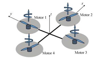
The quad-rotor has two pairs of propellers (1, 3) and (2, 4) with four motors, described in Fig. 1.
|
Figure 1 Structure of a quad-rotor aircraft |
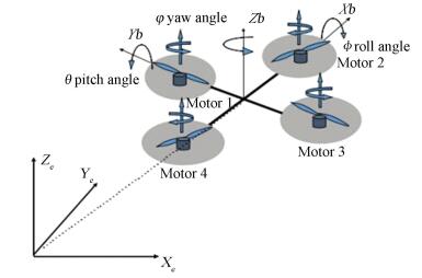
The structure is symmetrical.The front and rear motors rotate anti-clockwise while the other motors rotate clockwise[20]. The quad-rotor aircraft has two frames, one is the inertial frame E(Xe, Ye, Ze) and the other is the body fixed frame B(Xb, Yb, Zb) with an origin in the center of the mass, as shown in Fig. 2.
|
Figure 2 The schematic representation of a quad-rotor aircraft |
The dynamic model is based on the following assumptions:
1) The fuselage is considered as rigid body with symmetrical structure.
2) The origin of the vehicle fixed frame and the center of mass are coincident.
3) The propellers are rigid in planar analysis.
Then it is reasonable to consider the fuselage as rigid in space, and the aerodynamic forces generated by the rotation of the propellers are added to it[21-22].
The absolute transnational position of the aircraft is described by W(x, y, z) and its attitude by the Euler angle η(ϕ, θ, φ), used corresponding to aeronautical convention, the convention matrix is:
| $ \mathit{\boldsymbol{R}} = \left[ {\begin{array}{*{20}{c}} {{{\rm{c}}_\varphi }{{\rm{c}}_\theta }}&{ - {{\rm{s}}_\varphi }{{\rm{c}}_\phi } + {{\rm{c}}_\varphi }{{\rm{s}}_\theta }{{\rm{s}}_\phi }}&{{{\rm{s}}_\phi }{{\rm{s}}_\varphi } + {{\rm{c}}_\varphi }{{\rm{s}}_\theta }{{\rm{c}}_\phi }}\\ {{{\rm{s}}_\varphi }{{\rm{c}}_\theta }}&{{{\rm{c}}_\varphi }{{\rm{c}}_\phi } + {{\rm{s}}_\varphi }{{\rm{s}}_\theta }{{\rm{s}}_\phi }}&{ - {{\rm{c}}_\varphi }{{\rm{s}}_\phi } + {{\rm{s}}_\varphi }{{\rm{s}}_\theta }{{\rm{c}}_\phi }}\\ { - {{\rm{s}}_\theta }}&{{{\rm{c}}_\theta }{{\rm{s}}_\phi }}&{{{\rm{c}}_\theta }{{\rm{c}}_\phi }} \end{array}} \right] $ | (20) |
where cθ stands for cos θ and sθ for sin θ.
Each propeller generates vertical lifting force, denoted as Fj=bΩj2, (j=1, 2, 3, 4), the overall lifting force T will be:
| $ T = \sum\limits_{j = 1}^4 {{F_j}} = b\sum\limits_{j = 1}^4 {\mathit{\Omega }_j^2} $ | (21) |
where b is the thrust factor; Ωj means the rotation rate of j propeller. Then the external force equation of quad-rotor aircraft is:
| $ m\left[ {\begin{array}{*{20}{c}} {\ddot x}\\ {\ddot y}\\ {\ddot z} \end{array}} \right] = \mathit{\boldsymbol{G}}\left[ {\begin{array}{*{20}{c}} 0\\ 0\\ 1 \end{array}} \right] - \mathit{\boldsymbol{RT}}\left[ {\begin{array}{*{20}{c}} 0\\ 0\\ 1 \end{array}} \right] $ | (22) |
where G means gravity of the quad-rotor aircraft. Substituting Eqs. (20) and (21) into Eq. (22), it can be got as:
| $ \left[ {\begin{array}{*{20}{c}} {\ddot x}\\ {\ddot y}\\ {\ddot z} \end{array}} \right] = \left[ \begin{array}{l} \frac{T}{m}\left( {{{\rm{s}}_\phi }{{\rm{s}}_\varphi } + {{\rm{c}}_\phi }{{\rm{c}}_\theta }{{\rm{c}}_\varphi }} \right)\\ \frac{T}{m}\left( { - {{\rm{c}}_\phi }{{\rm{s}}_\varphi } + {{\rm{s}}_\phi }{{\rm{c}}_\theta }{{\rm{c}}_\varphi }} \right)\\ - g + \frac{T}{m}\left( {{{\rm{c}}_\varphi }{{\rm{c}}_\theta }} \right) \end{array} \right] $ | (23) |
Based on the earth-fixed inertial frame E, the generalized torques (yawing moment, pitching moment and rolling moment) can be written as:
| $ {\mathit{\boldsymbol{\tau }}_g} = \left[ {\begin{array}{*{20}{c}} {{\tau _\phi }}\\ {{\tau _\theta }}\\ {{\tau _\varphi }} \end{array}} \right] = \left[ {\begin{array}{*{20}{c}} {lb\left( {\mathit{\Omega }_4^2 - \mathit{\Omega }_2^2} \right)}\\ {lb\left( {\mathit{\Omega }_3^2 - \mathit{\Omega }_1^2} \right)}\\ {d\left( {\mathit{\Omega }_2^2 + \mathit{\Omega }_4^2 - \mathit{\Omega }_1^2 - \mathit{\Omega }_3^2} \right)} \end{array}} \right] $ | (24) |
where τϕ, τθ, τφ mean the three-axis torques caused by brush-less motors; l denotes the distance from the motors to the center of the aircraft; d is the torque coefficient. The gyroscopic torques is:
| $ {\mathit{\boldsymbol{\tau }}_G} = \left[ {\begin{array}{*{20}{c}} {{\tau _{{\rm{gyro}},{j_x}}}}\\ {{\tau _{{\rm{gyro}},{j_y}}}}\\ {{\tau _{{\rm{gyro}},{j_z}}}} \end{array}} \right] = \left[ {\begin{array}{*{20}{c}} {{{\vec w}^ * }{J_r}{\mathit{\Omega }_{j_x}}}\\ {{{\vec w}^ * }{J_r}{\mathit{\Omega }_{j_y}}}\\ {{{\vec w}^ * }{J_r}{\mathit{\Omega }_{j_z}}} \end{array}} \right] $ | (25) |
| $ {\mathit{\boldsymbol{J}}_r} = \left[ {\begin{array}{*{20}{c}} {{J_{rx}}}&0&0\\ 0&{{J_{ry}}}&0\\ 0&0&{{J_{rz}}} \end{array}} \right] $ | (26) |
So the torques function of quad-rotor has:
| $ \mathit{\boldsymbol{I}}\dot \eta = - {\eta ^ * }\mathit{\boldsymbol{I}}\eta + {\mathit{\boldsymbol{\tau }}_g} + {\mathit{\boldsymbol{\tau }}_G} $ | (27) |
This yield:
| $ \left[ {\begin{array}{*{20}{c}} {\ddot \varphi }\\ {\ddot \theta }\\ {\ddot \varphi } \end{array}} \right] = \left[ {\begin{array}{*{20}{c}} {\frac{{{J_y} - {J_z}}}{{{J_x}}}qr + \frac{{{J_{rz}}}}{{{J_x}}}\delta q + \frac{{{\tau _\varphi }}}{{{J_x}}}}\\ {\frac{{{J_z} - {J_x}}}{{{J_y}}}pr - \frac{{{J_{rz}}}}{{{J_y}}}\delta p + \frac{{{\tau _\theta }}}{{{J_y}}}}\\ {\frac{{{J_x} - {J_y}}}{{{J_z}}}pq + \frac{{{\tau _\phi }}}{{{J_z}}}} \end{array}} \right] $ | (28) |
where δ=(Ω1-Ω2+Ω3-Ω4).
Here, the artificial input variables are set as follows:
| $ \left\{ \begin{array}{l} {u_1} = b\left( {\omega _1^2 + \omega _2^2 + \omega _3^2 + \omega _4^2} \right)\\ {u_2} = b\left( {\omega _4^2 - \omega _2^2} \right)\\ {u_3} = b\left( {\omega _3^2 - \omega _1^2} \right)\\ {u_4} = d\left( {\omega _2^2 + \omega _4^2 - \omega _1^2 - \omega _3^2} \right) \end{array} \right. $ | (29) |
So, the dynamical model of a Quad-rotor aircraft is described as follows:
| $ \left[ {\begin{array}{*{20}{c}} {\ddot x}\\ {\ddot y}\\ {\ddot z}\\ {\ddot \varphi }\\ {\ddot \theta }\\ {\ddot \phi } \end{array}} \right] = \left[ {\begin{array}{*{20}{c}} {\frac{{{u_1}}}{m}\left( {{{\rm{s}}_\phi }{{\rm{s}}_\varphi } + {{\rm{c}}_\phi }{{\rm{c}}_\theta }{{\rm{c}}_\varphi }} \right)}\\ {\frac{{{u_1}}}{m}\left( { - {{\rm{c}}_\phi }{{\rm{s}}_\varphi } + {{\rm{s}}_\phi }{{\rm{c}}_\theta }{{\rm{c}}_\varphi }} \right)}\\ { - g + \frac{T}{m}\left( {{{\rm{c}}_\varphi }{{\rm{c}}_\theta }} \right)}\\ {\frac{{{J_y} - {J_z}}}{{{J_x}}}qr + \frac{{{J_{rz}}}}{{{J_x}}}\delta q + \frac{{{u_2}}}{{{J_x}}}}\\ {\frac{{{J_z} - {J_x}}}{{{J_y}}}pr - \frac{{{J_{rz}}}}{{{J_y}}}\delta p + \frac{{{u_3}}}{{{J_y}}}}\\ {\frac{{{J_x} - {J_y}}}{{{J_z}}}pq + \frac{{{u_4}}}{{{J_z}}}} \end{array}} \right] $ | (30) |
After analyzing the TS-fuzzy SVR algorithm and the model of the quad-rotor, an inverse model controller is put forward to the attitude system of the quad-rotor aircraft. Controllers are connected in series to the Quad-rotor, as shown in Fig. 3.

|
Figure 3 Inverse model control-based TS-fuzzy SVR combined with PID for quad-rotor aircraft |
In Fig. 3, r(t) is reference input of the attitude system of the quad-rotor; y(t) is system output; ua(t) and ub(t) are controller outputs of the PID controller and TS-fuzzy SVR inverse controller, respectively.
In order to determine the attitude system model, taking random signals as the input of the system to stimulate the attitude system, and subsequently get 1 000 input-output data as the training data. The system can be viewed as consisting of θ, φ, ϕ (the output of quad-rotor angles), u2, u3, u4 (the input control variables) and p, q, r (the attitude angular velocity). The mathematical model can be expressed as follows.
| $ \begin{array}{l} \left[ \begin{array}{l} \theta \left( {t + 1} \right)\\ \varphi \left( {t + 1} \right)\\ \phi \left( {t + 1} \right) \end{array} \right] = \\ \;\;\;\;\;SVR\left[ {\begin{array}{*{20}{c}} {q\left( {t - 1} \right)}&{r\left( {t - 1} \right)}&{{u_2}\left( t \right)}\\ {p\left( {t - 1} \right)}&{r\left( {t - 1} \right)}&{{u_3}\left( t \right)}\\ {q\left( {t - 1} \right)}&{p\left( {t - 1} \right)}&{{u_4}\left( t \right)} \end{array}} \right] \end{array} $ | (31) |
Then the corresponding TS-fuzzy SVR internal model controller is:
| $ \begin{array}{l} \left[ \begin{array}{l} {u_2}\left( t \right)\\ {u_3}\left( t \right)\\ {u_4}\left( t \right) \end{array} \right] = \\ \;\;\;\;\;SVR\left[ {\begin{array}{*{20}{c}} {q\left( {t - 1} \right)}&{r\left( {t - 1} \right)}&{\theta \left( {t - 1} \right)}\\ {p\left( {t - 1} \right)}&{r\left( {t - 1} \right)}&{\varphi \left( {t - 1} \right)}\\ {q\left( {t - 1} \right)}&{p\left( {t - 1} \right)}&{\phi \left( {t - 1} \right)} \end{array}} \right] \end{array} $ | (32) |
where θ(t+1), φ(t+1), ϕ(t+1) are predictions of the expected output values. Because the coupling coefficient with the attitude system of Quad-rotor is small, in this paper the attitude system is divided into three subsystems, roll, yaw and pitch. Here selecting the pitch subsystem as an example, firstly x(t)=[q(t-1), r(t-1), θ(t-1)] and y(t)=u2(t) will be regarded as the regression vectors, and then the TS-fuzzy SVR inverse controller model can be trained with {x(t), y(t)}t=11000.
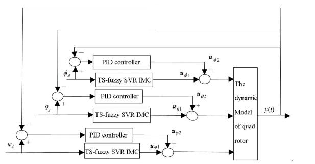
The system structure of IMC based on TS-fuzzy SVR is shown in Fig. 4.
|
Figure 4 Attitude control system-based TS-fuzzy SVR IMC combined with PID for quad-rotor aircraft |
In Fig. 4, ϕd, θd, φd are reference input of the attitude system of the Quad-rotor; y(t) is system output, including Euler angle, angular rate and angular derivative rate; uϕ1, uϕ2, uθ1, uθ2 and uφ1, uφ2 are controller output of the PID controller and TS-fuzzy SVR inverse controller, respectively.
4 SimulationIn this section, a controller combined with TS-fuzzy SVR inverse model controller and PID controller will be simulated in the quad-rotor aircraft model. The simulations were implemented using the SV-Machine Matlab Toolbox 1.0[23].
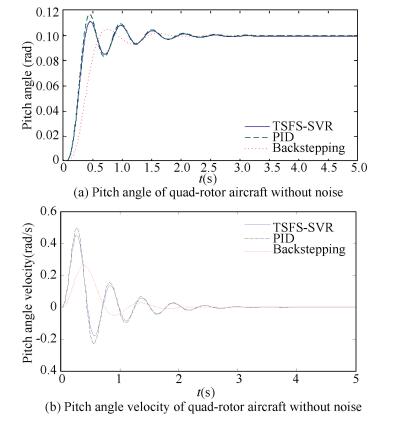
According to Eqs. (31) and (32), the controller combined with TS-fuzzy SVR inverse model controller and PID controller is shown in Fig. 3. And the simulations are carried out to verify the interference refection ability, fast responsiveness and reliability of the system by using MATLAB.Here two other controllers (PID controller and Backstepping controller) to observe the control ability and interference rejection ability of the new proposed controller (a controller combined with TS-fuzzy SVR inverse model controller and PID controller), where the Backstepping controller has already widely studied in quad-rotor aircrafts.The parameters of PID controller were be the same as the PID controller in the proposed controller, where p=120, i=0.2, d=27. The each channel parameters of Backstepping control law are chosen as follows:k1=4.2, k2=1.8, k3=3.9, k4=2.0, k5=4.7, k6=1.7. The coupling coefficients among the three channels are small, so the pith channel is focused on in the next simulations. The initial pitch angle is set to 0 rad and the target pitch angle is 0.1 rad. The simulation time is 5 s.
The simulation firstly considered the control process without noise interference. According to the simulation results, from Fig. 5, all the three kinds of controllers can achieve the proposed output. Backstepping control obtained the smallest overshoot (p=0.02) and the biggest rise time (tr=0.58 s).PID control obtained the biggest overshoot (p=0.18) and the smallest rise time (tr=0.27 s). And the proposed controller with TS-fuzzy SVR(TSFS) got a smaller overshoot (p=0.11) than PID controller, a smaller rise time (ts=0.271 s) than Backstepping controller. Also these differences can be seen from Fig. 5(b) accordingly.
|
Figure 5 Results of three controllers without noise |
To test the robustness of the new proposed controller with TS-fuzzy SVR, two groups of simulations were done for the three controllers. Firstly, a Gaussian noise was added to the dynamics equations of the Quad-rotor with mean zero and standard deviation 0.2. Seen from Figs. 6(a) and 6(b), Backstepping controller could not get a convergent output, but PID controller and the new proposed controller achieved the expected output, and the proposed controller with TS-fuzzy SVR got a smaller overshoot than PID controller.
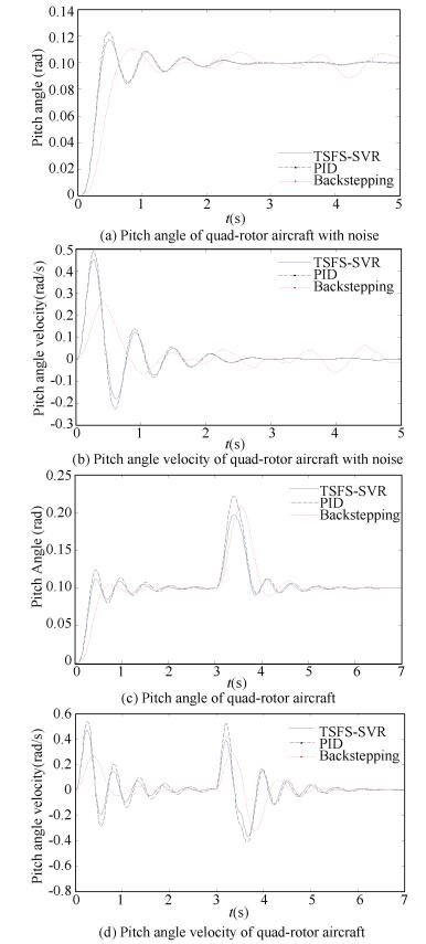
|
Figure 6 Results of three controllers with noise |
In the second set of simulations, a step noise was added to the inputs of quad-rotor after the outputs of the Quad-rotor been the expected value, which was 0.1 amplitude, lasted 0.5 s. Figs. 6(c) and 6(d) show that the three kinds of controllers made a prompt response and achieved the expected value, while the new proposed controller with TS-fuzzy SVR got a smallest overshoot, and a slower response time than Backstepping controller.
Since it is not easy to obtain the actual dynamic equations of Quad-rotor, here the model in the simulations is a simplified approximately linear model. PID controller has good control ability for the linear system. So the control of PID was similar to the proposed controller's control. However, in contrast, the new controller has the advantage in complex nonlinear system, and the prospect of the new controller is more promising in the practical application.
5 ConclusionsThis paper proposes an IMC scheme based on TS-fuzzy support vector regression for the attitude angles control of a quad-rotor aircraft. The number of kernel parameters in TS-fuzzy SVR is determined by the clustering approach that gets a high generalization ability and robustness by a linear SVR. Combing with the TS-fuzzy SVR, an inverse model controller is built. To construct a closed-loop feedback control system, a PID controller is added to the inverse model controller. The simulation results show that the proposed controller for a quad-rotor aircraft has a better interference rejection ability, fast responsiveness and reliability than PID controller and Backstepping controller.
| [1] |
Rinaldi F, Chiesa S, Quagliotti F. Linear quadratic control for quadrotors UAVs dynamics and formation flight. Journal of Intelligent & Robotic Systems, 2013, 70(1-4): 203-220. ( 0) 0)
|
| [2] |
dos Santos S R B, Nascimento C L, Givigi S N. Design of attitude and path tracking controllers for quad-rotor robots using reinforcement learning. 2012 IEEE Aerospace Conference. Piscataway: IEEE, 2012. 1-16. DOI: 10.1109/AERO.2012.6187314.
( 0) 0)
|
| [3] |
Li J S, Song L B, Yan G Z. Attitude control for small unmanned four-rotor based on adaptive inverse control. Journal of Shanghai Jiaotong University, 2012, 46(6): 89-93. ( 0) 0)
|
| [4] |
Zhao Zhicheng, Liu Zhiyuan, Xia Zhimin, et al. Internal model control based on LS-SVM for a class of nonlinear process. Physics Procedia, 2012, 25: 1900-1908. DOI:10.1016/j.phpro.2012.03.328 ( 0) 0)
|
| [5] |
Lin C T, Liang S F, Yeh C M, et al. Fuzzy neural network design using support vector regression for function approximation with outliers. 2005 IEEE International Conference on Systems, Man and Cybernetics. Piscataway: IEEE, 2005, 3: 2763-2768. DOI: 10.1109/ICSMC.2005.1571568.
( 0) 0)
|
| [6] |
Vapnik V. The Nature of Statistical Learning Theory. New York: Springer Science & Business Media, 2013, 17-30.
( 0) 0)
|
| [7] |
Juang C F, Hsieh C D. TS-fuzzy system-based support vector regression. Fuzzy Sets and Systems, 2009, 160(17): 2486-2504. DOI:10.1016/j.fss.2008.11.022 ( 0) 0)
|
| [8] |
Ji R, Yang Y, Zhang W. Incremental smooth support vector regression for Takagi-Sugeno fuzzy modeling. Neurocomputing, 2014, 123: 281-291. DOI:10.1016/j.neucom.2013.07.017 ( 0) 0)
|
| [9] |
Rossi F, Villa N. Support vector machine for functional data classification. Neurocomputing, 2006, 69(7-9): 730-742. DOI:10.1016/j.neucom.2005.12.010 ( 0) 0)
|
| [10] |
Ji R, Yang Y, Zhang W. TS-fuzzy modeling based on ε-insensitive smooth support vector regression. Journal of Intelligent & Fuzzy Systems: Applications in Engineering and Technology, 2013, 24(4): 805-817. DOI:10.3233/IFS-2012-0599 ( 0) 0)
|
| [11] |
Schölkopf B, Smola A J, Williamson R C, et al. New support vector algorithms. Neural Computation, 2000, 12(5): 1207-1245. DOI:10.1162/089976600300015565 ( 0) 0)
|
| [12] |
Williams C K I. Learning with kernels: Support vector machines, regularization, optimization, and beyond. Journal of the American Statistical Association, 2003, 98(3): 489-489. ( 0) 0)
|
| [13] |
Wang H, Pi D, Sun Y. Online SVM regression algorithm-based adaptive inverse control. Neurocomputing, 2007, 70(4-6): 952-959. DOI:10.1016/j.neucom.2006.10.021 ( 0) 0)
|
| [14] |
Bhandari S, Chen B, Colgren R, et al. Application of support vector machines to the modeling and control of a UAV helicopter. AIAA Modeling and Simulation Technologies Conference and Exhibit. Reston, VA : AIAA, 2007. 6708-6710. DOI: 10.2514/6.2007-6708.
( 0) 0)
|
| [15] |
Shin J, Kim H J, Kim Y. Adaptive support vector regression for UAV flight control. Neural Networks, 2011, 24(1): 109-120. DOI:10.1016/j.neunet.2010.09.011 ( 0) 0)
|
| [16] |
D'Urso P. Fuzzy clustering for data time arrays with inlier and outlier time trajectories. IEEE Transactions on Fuzzy Systems, 2005, 13(5): 583-604. DOI:10.1109/TFUZZ.2005.856565 ( 0) 0)
|
| [17] |
Guo Z K, Song Z Q, Mao J Q. An improved online least squares support vector machines regression algorithm. Control and Decision, 2009, 24(1): 145-148. ( 0) 0)
|
| [18] |
Zhang J S, Leung Y W. Robust clustering by pruning outliers. IEEE Transactions on Systems, Man, and Cybernetics, Part B: Cybernetics, 2003, 33(6): 983-998. DOI:10.1109/TSMCB.2003.816993 ( 0) 0)
|
| [19] |
Liu Y N, Zhang S X, Cao L J, et al. Nonlinear robust adaptive flight controller design based on LS-SVM. Systems Engineering and Electronics, 2012, 34(12): 2541-2547. ( 0) 0)
|
| [20] |
Cavalcante Sa R, De Araujo A L C, Varela A T, et al. Construction and PID control for stability of an unmanned aerial vehicle of the type quadrotor. Robotics Symposium and Competition (LARS/LARC), 2013 Latin American. Pisacataway: IEEE, 2013. 95-99. DOI: 10.1109/LARS.2013.64.
( 0) 0)
|
| [21] |
Bergamasco M, Lovera M. Identification of linear models for the dynamics of a hovering quadrotor. IEEE Transactions on Control Systems Technology, 2014, 22(5): 1696-1707. DOI:10.1109/TCST.2014.2299555 ( 0) 0)
|
| [22] |
Oosedo A, Konno A, Matsumoto T, et al. Design and attitude control of a quad-rotor tail-sitter vertical takeoff and landing unmanned aerial vehicle. Advanced Robotics, 2012, 26(3-4): 307-326. DOI:10.1163/156855311X614590 ( 0) 0)
|
| [23] |
Chang C C, Lin C J. LIBSVM: A library for support vector machines. ACM Transactions on Intelligent Systems and Technology (TIST), 2011, 2(3): 27-28. ( 0) 0)
|
 2017, Vol. 24


