The challenge to achieve a win-win situation where high quality and low cost are both attained has received a broad spectrum of interest from academia and industry, especially in the semiconductor manufacturing that is generally recognized as the most complex system with extremely expensive equipment[1-2].
Jobs of similar types are grouped into a family, which is viewed as a leverage to decrease setup times, reduce lead time as well as increase equipment utilization[3-4]. Various academic achievements have been made to analyze family scheduling problems in semiconductor manufacturing systems. For instance, Chern et al.[5]investigated the effect of applying family-based scheduling rules to wafer fabrication and then presented five family-based rules. Zheng et al.[6] dealt with an unbounded batching machine scheduling problems with family jobs and setup times by developing a generic forward dynamic programming algorithm. Yugma et al.[7] proposed a heuristic algorithm for solving a batching and scheduling problem in semiconductor diffusion.
All the above-mentioned literatures fail to consider the practical production case where machine parameters may drift after a certain quantity of job processing especially in high mixed fabs[8]. To guarantee high quality, a qualification run (qual-run) is regarded as an indispensable operation to evaluate machine status, ensuring that the machine is qualified to process the jobs of a certain family[9-10]. Currently, little attention is paid to considering the qual-run as a significant constraint which may directly affect the scheduling. Li et al.[11] analyzed the impact of qual-run requirements on the scheduling performance and proved through simulation results that more jobs make a greater impact on the performance. Patel[12] proposed four heuristics to solve the problem of scheduling of job families on non-identical parallel machines with qual-run constraints.
As shown above, there are several existing works covering qual-run requirements, however, qual-runs and setups are not taken as two main contradictory constraints. Owing to the fact that taking the qual-run into consideration is important and imperative in real life, a single machine multi-family problem with an objective of minimizing makespan was addressed, which took setups and qual-runs as two closely interactive constraints. Since the problem-solving methods of the abovementioned literatures are inappropriate to figure out the problem, an adaptive catastrophic differential evolution algorithm with depth neighborhood search was proposed. Differential evolution with its advantage of superior global optimization ability and convenient operation is popularly and successfully employed in a wide range of fields[13-16]. The proposed algorithm, preserving these characteristics and making up for the deficiency of easily trapping in local optimum and poor local search ability, demonstrates its exceptional performance in solving the following problem.
2 Problem DescriptionIn this paper, a single machine scheduling problem with multi-family cases where there are M jobs that belong to F families required to be processed on a machine was presented. Switching from one job to another of a different family requires setups, and one effective way to avoid the setup is to process as more jobs as possible in a row, while a qual-run is incurred if jobs of other families have been processed for a predefined limited number since the last time the job of the same family was processed. In other words, if the number of processed jobs that are from other families exceeds a qual-run threshold of the family, a qual-run is triggered. Moreover, it is notable that a qual-run operation usually takes a relatively long time, which makes it economically wise to avoid performing a great number of qual-runs. Given this, the paper strives to strike a balance between the qual-run and setup times with an objective to minimize makespan.
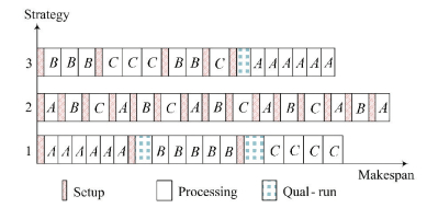
To clearly state the problem, an illustrative example is given in Fig. 1 with three scheduling strategies. Assume that there are three families A, B, C, the numbers of jobs in them are 6, 5 and 4 with qual-run thresholds being 2, 3 and 3, respectively.
|
Figure 1 An illustrative example for scheduling with the qual-run |
Solution 1 is a regular scheduling mode of processing all jobs of the same family in a successive way without deliberately avoiding qual-runs. Solution 2 goes to great lengths to avert qual-runs and solution 3 is a merger of the first two solutions. It is evident in Fig. 1 that Solution 3 performs best among the three solutions. It finds out a balance between setup and qual-run times, instead of blindly avoiding qual-runs or setups alone.
In order to form the precise problem domain, the hypotheses are made as follows: 1) One machine can process at most one job at a time, and preemption of processing is not allowed. 2) Jobs of the same family have the same processing time. 3) All jobs are available at the very beginning in the schedule. 4) The setup time is sequence-independent and no setup is required between jobs of the same family. 5) A setup is executed before a qual-run. 6) A qual-run is unnecessary for the very first job.
To state the problem clearly, the following notations are defined, as shown in Table 1.
| Table 1 Notation definition |
Based on the assumption and Ref.[10], the mathematical model of the problem is formulated as follows:
| $ \min {C_{\max }} $ | (1) |
| $ \sum\limits_{j \in J} {{P_{j\left( f \right)i}}} \le 1,\forall i \in I $ | (2) |
| $ \sum\limits_{j \in J} {{P_{j\left( f \right)i}}} \le {m_f},\forall f \in F $ | (3) |
| $ {P_{f\left( j \right)i}} - {P_{f\left( j \right)\left( {i - 1} \right)}} \le {S_{f\left( j \right)i}},\forall f \in F,\forall j \in J,\forall i \in I $ | (4) |
| $ \begin{array}{l} {P_{f\left( j \right)i}} - \sum\limits_{i' = i - {n_f}}^{i - 1} {{P_{f\left( j \right)i'}}} \le {Q_{f\left( j \right)i}},\forall f \in F,\forall j \in J,\\ \;\;\;\;\;\;\;\;\forall i \in I \end{array} $ | (5) |
| $ \begin{array}{l} {C_{i - 1}} + {P_{f\left( j \right)i}} \cdot {p_f} + {S_{f\left( j \right)i}} \cdot {s_f} + {Q_{f\left( j \right)i}} \cdot {q_f} = {C_i},\\ \;\;\;\;\;\;\;\forall i \in I \end{array} $ | (6) |
Objective 1) represents minimizing makespan. Constraint 2) ensures that a position can process at most one job. Constraint 3) restricts the total number of jobs of each family. Constraint 4) decides whether family f requires a setup. Constraint 5) decides whether family f requires a qual-run. Constraint 6) guarantees that the job should be processed instantly after the completion of the job in the last position.
The solution that all jobs of the same family are processed in a row meets the above criteria. It is viewed as an original and primitive solution. In this solution, all families except the family of the first job in the schedule are required to execute qual-runs, as we can see, all possible setups are reduced, and the qual-run times of those families are 1. Therefore, the only way to find a better solution is to ensure that the number of qual-runs of each family is not more than one, as shown in Formula (7).
| $ \sum\limits_{j = 0}^J {{Q_{j\left( f \right)i}}} \le 1,\forall f \in F,\forall i \in I $ | (7) |
Formula (7) implies that some families are qual-run free, and some have to execute qual-runs. Which certain families to choose from to avoid the qual-run is the pillar and ground of this study. Consequently, a definition is presented.
Definition 1 Block: Families to be scheduled are spilt into two types of blocks. Batches in Block 1 (B1) are qual-run free, which means no qual-run is needed between two batches, while batches in Block 2 (B2) require qual-runs.
Definition 1 provides a fundamental theoretic basis of the scheduling. Thus, if the solution obtained goes against the concept of Definition 1, it will not be regarded as feasible in the following sections. It is also notable that B1 is certainly scheduled before B2. Since if B2 is executed before B1, it is impossible that all jobs of families in B1 can be spared from qual-runs. Since B1 must be processed first, the number of each type of block is set to 0 or 1, which is good enough for operating easily and comprehending clearly.
In view of families in blocks, the following properties are obtained.
Property 1 Only when families in B1 and B2 are not overlapped is the solution near optimal.
Proof For jobs of a family, there are only three sets of assignment ways. Set 1: Both B1 and B2 have jobs of family f. Set 2: Only B2 has jobs of family f. Set 3: Only B1 has jobs of family f. For Set 1, family f in B1 is out of qual-runs, while the one in B2 requires qual-runs, so the total setup and qual-run time (t1) is lf·sf+qf. For Set 2, the total setup and qual-run time (t2) is sf+qf, less than t1. For Set 3, if the total setup and qual-run time (t3) is more than t1, Set 2 is better. If t3≤t1, Set 2 or 3 is better. All in all, either Set 2 or 3 invariably performs better than Set 1. Therefore, only when families in B1 and B2 are not overlapped is the solution near optimal.
An excellent scheduling of the problem features that as few setups as possible are performed and as many qual-runs as possible are averted. As shown in Definition 1, all families in B2 are supposed to execute qual-runs, so it's better to continuously process all jobs of the same family in B2 to avoid extra setups. So, the difficulty and key point of the study focus on B1, instead of B2. Thanks to the help of Property 1, the scheduling difficulty is reduced. The scheduling is simplified to two main tasks, one is to determine the member of B1, B2 and another is to consider the appropriate batch size of families in B1 to avoid qual-runs.
Definition 2 Periodic scheduling scheme: a pattern of the batch size of each family in B1. For instance, period 1 includes all families assigned to B1. With the scheduling process moving on, jobs of a certain family may be exhausted, then the next period is prepared and batch sizes of the rest of families are recalculated.
Property 2 A feasible solution is possible to obtain when families in B1 satisfy the following relation.
| $ \sum\limits_{f \in {B_1}\backslash \left\{ k \right\}} {{E_f} \le {n_k}} ,k \in {B_1} $ | (8) |
Proof For any family, it is prerequisite to satisfy that the number of jobs between the last job in the last batch and the first job in this batch, namely, the sum of batch sizes of other families, does not exceed the threshold of the family. Fig. 2 simplifies the problem to three families. Choose a part of one period, and it is plain to see that every family in B1 can avoid qual-runs by satisfying

|
Figure 2 An illustrative example of batch sizes in B1 |
Theorem 1 The batch sizes of families in B1 are required to satisfy the following formula, which develops a feasible solution for B1 to avoid the qual-run.
| $ E_f^v \ge \max \left\{ {\left( {v - {n_f}} \right),1} \right\},f \in {B_1} $ | (9) |
where v represents the number of jobs processed in a pattern and Efv means the batch size of family f when the number of jobs processed in a pattern is v.
Proof Ensuring that all families have been processed in the pattern can avoid qual-runs, the sum of jobs processing in B1 must be at least NB1. Formula (9) can be attained by Property 2, if
Theorem 2 The number of families in B1(NB1) which meets Formula (10) can generate a feasible solution for B1.
| $ {N_{{B_1}}} \le \min {n_{j \in {B_1}}} + 1,0 \le {N_{{B_1}}} \le N $ | (10) |
Proof Given that the number of the families in B1 reaches the maximum, the batch sizes of all families in B1 are supposed to be 1, which makes B1 have the maximal capacity. The number of jobs between the last job to the next job of this family is limited to min nj∈B1, meanwhile, batch sizes of all families in B1 are 1, so NB1(max)=min nj∈B1+1. Batch sizes of all families in B1 may not all equal 1, so NB1≤min nj∈B1+1.
Theorem 3 The maximum of the sum of the batch sizes (vmax) in a pattern satisfies Formula (11).
| $ {v_{\max }} = v,{\rm{if}}\sum\limits_{f = 1}^{{N_{{B_1}}}} {E_{f\left( {\min } \right)}^v} \le v,\sum\limits_{f = 1}^{{N_{{B_1}}}} {E_{f\left( {\min } \right)}^{v + 1}} > v + 1 $ | (11) |
Proof As
Since the multi-family scheduling problem with qual-run and setup constraints in a single machine case is an NP-hard problem[10], the exactly accurate solution on a large scale is hard to figure out. On the basis of the non-linear programming model, a modified adaptive catastrophic differential evolution algorithm with depth neighborhood search (MACDE) is put forward. The algorithm adopts a multi-tier encoding mechanism elaborating the scheduling scheme. With the help of the catastrophe theory and adaptive process, the disadvantage of differential evolution that the population is prone to be premature can be avoided and the speed of convergence can be accelerated[17-20].Moreover, armed with the depth neighborhood search, the algorithm conducts the deep-going search. The proposed hybrid differential evolution algorithm balances the exploration and exploitation, showing a strong optimization capability with a larger and deeper search scope and range. The details of the algorithm are listed as follows.
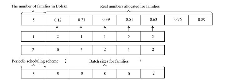
3.1 EncodingMulti-tier encoding is employed in the algorithm, as shown in Fig. 3. For better understanding, the first level is named as the main level, and the remaining levels are called the subsidiary level.
|
Figure 3 The schematic diagram of encoding representation |
In the main level, the first position of the code is a positive integer, expressing the family number in B1, the rest are real numbers in an increasing order. Each real number which represents a family is randomly assigned.
In the subsidiary levels, the first position represents the first periodic scheduling scheme, the rest show the batch size of each family. When jobs of a certain family are exhausted, the next level is prepared to be set up.
3.2 InitializationFirst, generate a target vector by randomly producing real numbers assigned for families between 0 and 1 and ranking the numbers in an increasing order, denoted by {Xr1, Xr2, Xr3, …, XrN}.
Second, adopting the concept of Theorem 2, it is easy to figure out at most how many families belong to B1.
Third, the initialization for batch sizes of families is performed, which requires to satisfy Theorems 1 and 3. Ensuring that v=Vmax is a better approach to diminish the searching range and speed up the exploration.
3.3 Fitness EvaluationBased on the objective of the paper, the fitness function can be obtained as below:
| $ {F_{{\rm{fit}}}} = \sum\limits_{f \in F} {\sum\limits_{j \in J} {\left( {{s_f} \cdot {S_{f\left( j \right)}} + {q_f} \cdot {Q_{f\left( j \right)}}} \right)} } $ | (12) |
The fitness value of each individual can be calculated by Formulas (4), (5) and (12).
3.4 Adaptive Mutation OperatorChoose a target vector of an individual of current population as a disturbance vector Xp1, rf, pick up two diverse individuals and treat Xp2, rf, Xp3, rf as two differential vectors. The mutation operation is carried out according to Formula (13).
| $ \begin{array}{l} {\mathit{\boldsymbol{Y}}_{{p_1},{r_f}}}\left( {G + 1} \right) = {\mathit{\boldsymbol{X}}_{{p_1},{r_f}}}\left( G \right) + {\delta _F} \cdot \left( {{\mathit{\boldsymbol{X}}_{{p_2},{r_f}}}\left( G \right) - } \right.\\ \;\;\;\;\;\;\;\;\;\;\;\;\;\;\;\;\;\;\;\;\left. {{\mathit{\boldsymbol{X}}_{{p_3},{r_f}}}\left( G \right)} \right) \end{array} $ | (13) |
where p1, p2, p3∈{1, …Pop}, p1≠p2≠p3, rf∈{1, 2, …, N}, Xp1, rf(G) represents the vector of family f of individual p1 in the Gth generation, δF is the adaptive mutation probability and calculated as Formula (14).
| $ {\delta _F} = \left\{ \begin{array}{l} \delta ,\;\;\;\;\;\;\;\;\;\;\;\;\;\;\;{\rm{if}}\;{\lambda _c} > \frac{\lambda }{3}\\ \min \left\{ {\frac{4}{{{\lambda _c}}},2} \right\},{\rm{if}}\;{\lambda _c} \le \frac{\lambda }{3} \end{array} \right. $ | (14) |
where λc signifies the countdown of catastrophe, λ is the catastrophe operator, and δ is the initial mutation probability.
3.5 Crossover OperatorA trial vector Zp1, rf(G+1) is produced according to Formula (15) that shows a recombination of the arget vector Xp1, rf(G) and the mutation vector Yp1, rf(G+1), and Zp1(G+1) is rearranged in an increasing order.
| $ \begin{array}{l} {\mathit{\boldsymbol{Z}}_{{p_1},{r_f}}}\left( {G + 1} \right) = \\ \;\;\;\;\;\;\;\left\{ \begin{array}{l} {\mathit{\boldsymbol{Y}}_{{p_1},{r_f}}}\left( {G + 1} \right),{\rm{if}}\;{R_{{r_f}}}\left( {0,1} \right) < {\mu _c},\;{\rm{or}}\;{r_f} = {r_{f\left( {{\rm{rand}}} \right)}}\\ {\mathit{\boldsymbol{X}}_{{p_1},{r_f}}}\left( G \right),\;\;\;\;\;\;{\rm{else}} \end{array} \right. \end{array} $ | (15) |
where μc represents the crossover probability, Rrf(0, 1) is a uniformly distributed random number for the rfth dimension, rf(rand) is a randomly selected integer between [1, N].
3.6 Depth Neighborhood SearchOn the basis of Theorems 1 and 3, the depth neighborhood search is carried out to redefine the batch sizes of families in B1.
Step 1 Let the periodic scheduling scheme (l) be 1. Let the count value (ccount) be 0.
Step 2 Let the sequence number of the family in B1 (k) be 1, and the number of the families in B1 is denoted by NB1.
Step 3 Set glk=
Step 4 Let a=g/1, if a=0, go to Step 5; otherwise, choose a of families from B1\{f}, add one job to the batch size.
Step 5 If f equals current number of families in B1 (Nf1), go to Step 7. If f≠Nf1, then f=f+1 and return to Step 3.
Step 6 Count the remainder jobs of each family, if jobs of a certain family are exhausted, then ccount=ccount+1.
Step 7 If ccount=Nf1, then l=l+1 and go to Step 2; otherwise, go to Step 8.
Step 8 The number of the families in B1 (N'B1) equals to N'B1-1, if N'B1=Nf1, then finish the neighborhood search; otherwise, return to Step 1.
3.7 Selecting OperatorCompare the target population and the trial population that are produced by a series of operations, and consequently choose the one with better fitness. The selecting operation can be described as follows:
| $ \begin{array}{l} {\mathit{\boldsymbol{O}}_{{p_1},{r_f}}}\left( {G + 1} \right) = \\ \;\;\;\;\;\;\;\left\{ \begin{array}{l} {\mathit{\boldsymbol{Z}}_{{p_1},{r_f}}}\left( {G + 1} \right),{\rm{if}}\;{F_{{\rm{fit}}}}\left( {{u_{{p_1}}}\left( {G + 1} \right)} \right) < {F_{{\rm{fit}}}}\left( {{x_{{p_1}}}\left( G \right)} \right)\\ {\mathit{\boldsymbol{X}}_{{p_1},{r_f}}}\left( G \right),\;\;\;\;\;\;{\rm{else}} \end{array} \right. \end{array} $ | (16) |
The catastrophe countdown λc is updated based on judging whether there emerges a new optimal solution, if yes, reset λc=λ, if not, λc=λc-1. When λc < 10, the mutation probability is adjusted, by which some characteristics of the previous evolutions can be maintained. When λc=0, the best individual can be retained, and then go back to reinitialize the population.
4 Experiments and AnalysisPerformance ratio (R) and computation time (T) constitute two criteria, evaluating the performance of the proposed algorithm effectively[21].
| $ \begin{array}{l} R = \\ \;\;\;\frac{{V\left( {H,T,Y} \right)}}{{\sum\limits_{f \in F} {\sum\limits_{j \in J} {{s_f} \cdot {S_{f\left( j \right)}}} } + \sum\limits_{f \in F} {\sum\limits_{j \in J} {{q_f} \cdot {Q_{f\left( j \right)}}} } - {q_{f\left( {\max } \right)}}}} \end{array} $ |
where V(H, T, Y) represents the result of problem instance Y solved by algorithm H in the Tth iteration, qf(max) is the maximal value of qual-run time among all families. The smaller the value is, the better the performance of the approach is. The computation time is determined by the complexity of the algorithm. The smaller the computation time is, the more efficient the algorithm is.
Programming language C++ is adopted on the basis of Visual Studio 2012 for the proposed algorithm. A computer with Intel Core i3 2.10 GHZ processor and 4 GB of main memory is adopted to conduct the following experiments.
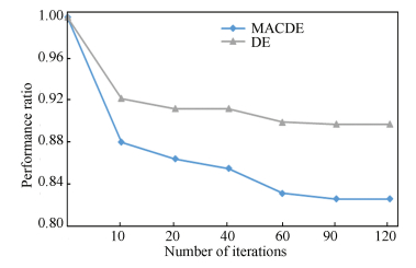
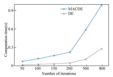
4.1 Parameters AnalysisUnder the situation where the number of families is 15, 30, instances are generated randomly, where the numbers of families are uniformly distributed between [3, 8], setup time is uniformly distributed between [1, 16], processing time is uniformly distributed between [50, 80], and qual-run time is equivalent with the value of the processing time. The proposed algorithm and the basic differential evolution algorithm (DE) are carried out to solve the problem instances and the corresponding results are shown in Figs. 4 and 5.
|
Figure 4 Number of iterations versus performance ratio for two algorithms |
|
Figure 5 Number of iterations versus computation time for two algorithms |
Fig. 4 shows that MACDE outperforms DE on the convergence performance. When the number of iterations is from 90 to 120, the solutions of the two algorithms are both tend to be stable. Fig. 5 displays that when the number of iterations grows to 200, the computation time increases precipitously. With a comprehensive of performance and computation time, it is reasonable to set the number of iterations be 100.
The other parameters are analyzed in the same manner with an extensive range of experiments that make use of varied values. The results demonstrate that the proper initial population size, the mutation probability, the crossover probability, the catastrophe frequency are 30, 0.3, 0.5, 10, respectively.
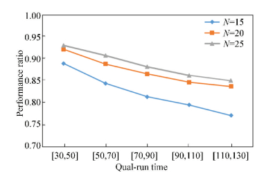
4.2 The Impact of Qual-run Constraints on Scheduling PerformanceSet the number of families respectively be 15, 20, 25 and maintain the values of other input parameters. Qual-run time is uniformly distributed between [30, 50], [50, 70], [70, 90], [90, 110], [110, 130]. The experimental results are shown in Fig. 6.
|
Figure 6 Relationship between qual-run time and performance ratio |
It is not hard to find from Fig. 6 that qual-run time is closely related to performance ratio. Generally, qual-run time lasts so long that a prominent scheduling approach that makes a trade-off between the qual-run and setup times is more important, which is best explained by Fig. 6.
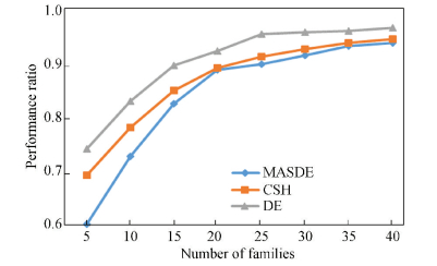
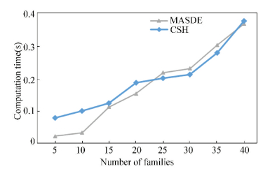
4.3 Comparisons Between Other AlgorithmsDue to the limitation of few studies considering qual-runs as well as setups, the structural heuristic algorithm (CSH) proposed by Cai et al.[10] is employed to serve as the benchmark for our problem under the same input parameters, and the comparative results are shown in Figs. 7 and 8.
|
Figure 7 Comparisons on performance ratio between DE, MASDE and CSH |
|
Figure 8 Comparisons on computation time between MACDE and Benchmark |
Fig. 7 displays that when the number of families is 15, MASDE has a distinct advantage over DE and CSH on the scheduling solution. With the number of families increasing, although the superiority is slipping, the competitive edge is still there. Similarly, as shown in Fig. 8, when the number of families is less than 20, the mutation time of MASDE is much less than that of CSH. When the number of families grows to 40, the computation time is roughly equal, however, with the number of families increasing, the computation time remains to be less than 0.5 s within a reasonable range. With a comprehensive consideration of performance ratio and computation time, a conclusion can be drawn that MASDE undoubtedly outperforms others. The reason can be firstly explained by that CSH is complemented based on each property on its own, however the four presented properties are supposed to be dependent and interactive. Secondly, due to its incomplete back search, CSH fails to obtain the optimal solution. All these shortcomings are overcome in MASDE and its novel search method is manifested to be effective both theoretically and practically.
5 ConclusionsThis paper studies a multi-family scheduling modeling of single machine at the backdrop of the semiconductor manufacturing system, considering qual-run constraints which are common in practical production and make a profound impact on machine utilization and production efficiency. An adaptive differential evolution based on catastrophe algorithm with depth neighborhood search is developed not only to resolve the problem but also to enrich the theoretical methods of the similar scheduling problem. Furthermore, the satisfying experimental results verify the validity and feasibility of the proposed algorithm. As future works, it is planned to develop the algorithm for optimizing problems in hybrid flow shops with more additional constraints, such as time constraints.
| [1] |
Akcalt E, Nemoto K, Uzsoy R. Cycle-time improvements for photolithography process in semiconductor manufacturing. IEEE Transactions on Semiconductor Manufacturing, 2001, 14(1): 48-56. DOI:10.1109/66.909654 ( 0) 0)
|
| [2] |
Zhou Binghai, Pan Qingzhi, Wang Shijing, et al. Modeling of photolithography process in semiconductor wafer fabrication systems using extended hybrid Petri nets. Journal of Central South University of Technology, 2007, 14(3): 393-398. DOI:10.1007/s11771-007-0077-1 ( 0) 0)
|
| [3] |
Sun Xiaoqing, Noble J S. An approach to job shop scheduling with sequence-dependent setups. Journal of Manufacturing Systems, 1999, 18(6): 416-430. DOI:10.1016/S0278-6125(00)87643-8 ( 0) 0)
|
| [4] |
Allahverdi A, Ng C T, Cheng T C E, et al. A survey of scheduling problems with setup times or costs. European Journal of Operational Research, 2008, 187(3): 985-1032. DOI:10.1016/j.ejor.2006.06.060 ( 0) 0)
|
| [5] |
Chern C C, Liu Y L. Family-based scheduling rules of a sequence-dependent wafer fabrication system. IEEE Transactions on Semiconductor Manufacturing, 2003, 16(1): 15-25. DOI:10.1109/TSM.2002.807742 ( 0) 0)
|
| [6] |
Zheng R, Li H, Zhang X. Scheduling an unbounded batching machine with family jobs and setups times. The Journal of the Operational Research Society, 2012, 63(2): 160-167. DOI:10.1057/jors.2010.187 ( 0) 0)
|
| [7] |
Yugma C, Dauzère-Pérès S, Artigues C, et al. A batching and scheduling algorithm for the diffusion area in semiconductor manufacturing. International Journal of Production Research, 2012, 50(8): 2118-2132. DOI:10.1080/00207543.2011.575090 ( 0) 0)
|
| [8] |
Rowshannahad M, Dauzere-Peres S, Cassini B. Capacitated qualification management in semiconductor manufacturing. Omega, 2015, 54: 50-59. DOI:10.1016/j.omega.2015.01.012 ( 0) 0)
|
| [9] |
Yugma C, Blue J, Dauzère-Pérès S, et al. Integration of scheduling and advanced process control in semiconductor manufacturing: review and outlook. Journal of Scheduling, 2015, 18(2): 195-205. DOI:10.1007/s10951-014-0381-1 ( 0) 0)
|
| [10] |
Cai Yiwei, Kutanoglu E, Hasenbein J, et al. Single-machine scheduling with advanced process control constraints. Journal of Scheduling, 2012, 15(2): 165-179. DOI:10.1007/s10951-010-0215-8 ( 0) 0)
|
| [11] |
Li Li, Qiao Fei. The impact of the qual-run requirement of APC on the scheduling performance in semiconductor manufacturing. Proceedings of the 2008 International Conference on Automation Science and Engineering. Piscataway: IEEE, 2008. 242-246. DOI: 10.1109/COASE.2008.4626542.
http://ieeexplore.ieee.org/document/4626542/
( 0) 0)
|
| [12] |
Patel N S. Lot allocation and process control in semiconductor manufacturing-A dynamic game approach. Proceedings of the 43rd IEEE Conference on Decision and Control. Piscataway: IEEE, 2004. 4234-4248. DOI: 10.1109/CDC.2004.1429418.
http://ieeexplore.ieee.org/xpls/icp.jsp?arnumber=1429418
( 0) 0)
|
| [13] |
Peng Wuliang, Huang Min. A critical chain project scheduling method based on a differential evolution algorithm. International Journal of Production Research, 2014, 52(13): 3940-3949. DOI:10.1080/00207543.2013.865091 ( 0) 0)
|
| [14] |
Feng Xiaoqiang, He Tiejun. Fast matching pursuit for traffic images using differential evolution. Journal of Harbin Institute of Technology (New Series), 2010, 17(2): 193-198. ( 0) 0)
|
| [15] |
Zhou Binghai, Hu Liman, Zhong Zhenyi. A hybrid differential evolution algorithm with estimation of distribution algorithm for reentrant hybrid flow shop scheduling problem. Neural Computing and Applications, 2016, 1-17. DOI:10.1007/s00521-016-2692-y ( 0) 0)
|
| [16] |
Onwubolu G, Davendra D. Scheduling flow shops using differential evolution algorithm. European Journal of Operational Research, 2006, 171(2): 674-692. DOI:10.1016/j.ejor.2004.08.043 ( 0) 0)
|
| [17] |
Wang Meng, Li Bixin, Wang Zhengshan, et al. An optimization strategy for evolution testing based on cataclysm. Proceedings of the 2010 IEEE 34th Annual Computer Software and Applications Conference Workshops. Piscataway: IEEE, 2010. 359-364. DOI: 10.1109/COMPSACW.2010.69.
http://ieeexplore.ieee.org/document/5614562/
( 0) 0)
|
| [18] |
Dong Chaojun, Liu Zhiyong, Qiu Zulian. Catastrophe-particle swarm optimization algorithm and its application to traffic control. Computer Engineering and Applications, 2005, 41(29): 19-23. ( 0) 0)
|
| [19] |
Li Xiangtao, Yin Minghao. Modified differential evolution with self-adaptive parameters method. Journal of Combinatorial Optimization, 2016, 31(2): 546-576. DOI:10.1007/s10878-014-9773-6 ( 0) 0)
|
| [20] |
Elsayed S M, Sarker R A, Essam D L. An improved self-adaptive differential evolution algorithm for optimization problems. IEEE Transactions on Industrial Informatics, 2013, 9(1): 89-99. DOI:10.1109/TII.2012.2198658 ( 0) 0)
|
| [21] |
Zhou Binghai, Wang Teng. Scheduling multiple orders per job with various constraints for hybrid flow shop. Control and Decision, 2016, 31(5): 776-782. DOI:10.13195/j.kzyjc.2015.0399 ( 0) 0)
|
 2018, Vol. 25


