 2018, Vol. 25


2. School of Mechanical Science & Engineering, Huazhong University of Science and Technology, Wuhan 430074, China
Modeling and representation of tolerances information have already become one of the most active and important research directions among the tolerance related research fields. In 3D CAD/CAPP/CAM system, modeling and representing tolerances information with a unified, unambiguous, both human and computer understandable mathematical model is the main task of tolerance modeling[1]. Over the last couple of decades, a great deal of efforts on tolerance modeling have been made and different kinds of tolerance models have been proposed, such as the offset model, the parametric model, the kinematic model, the Technologically and Topologically Related Surfaces (TTRS) model, the Tolerance-Map (T-Map) model and SDT model etc[2]. The offset model requires separate tolerance zones for each type of tolerances even on the same feature therefore it cannot handle interaction and couple of various tolerances and it is not conformant to the new generation GPS system. The parametric model is unable to implement geometric tolerances as it can only work with variation of dimensional parameters[3]. Chase et al.[4] developed a generalized method to implement assembly tolerance analysis considering the effects of all geometric feature variations. Marziale et al.[5] made a comprehensive comparison and gave their analogies and differences between the two models for tolerance analysis, namely the vector loop model and the matrix model. The TTRS model was developed by Desrochers and Clément[6] from the perspective of establishing the tolerances information represenation model independent of the modeling system. The idea of T-Maps was proposed for the first time in a NSF proposal by Davidson and Shah in 1998[3]. A Tolerance-Map can describe all variational possibilities in size, shape, orientation, and location of a target feature using a hypothetical Euclidean point space[7-8]. The T-Maps model for geometrical feature variations is based on basis tetrahedron and areal coordinates. Ameta et al.[9-10] extended T-Maps to implement the probabilistic representations of clearances and statistical allocation of tolerances. The SDT model uses three rotation vectors and three translation vectors to describe any small displacement of a rigid body. On the basis of SDT, Teissandier et al.[11] developed a 3D tolerance analysis tool using the Proportioned Assembly Clearance Volume. Desrochers et al.[12] suggested the torsor representations of almost all standard tolerance zones together with various standardized connections between any two rigid bodies. Laperrière et al.[13] proposed a comparative research between the Jacobian and screw based methods. Marziale et al.[14] proposed the unified Jacobian-torsor model to perform tolerance analysis, as an evolution model of the two existing models, by comparing the analogies and differences between the Jacobian model and the torsor model. Bo et al.[15] introduced three models of tolerance analysis—the Jacobian, the torsor and the vector loop, and made a comparative study on advantages, disadvantages and application scope of them. Ghie et al.[16-17] introduced a statistical tolerance analysis method which is performed based on the unified Jacobian-Torsor model, and then Zuo et al.[18] discussed the application of this model in error propagation analysis, Chen et al.[19] suggested a modified approach of this model taking into account the constraints between torsor components.
As mentioned above, most of the existing researches have focused on modeling of regular feature variations, very few researches have presented to carry out tolerance modeling of complex or irregular feature variations[1]. Furthermore, the most modeling theories are aimed at traditional GPS standards system or only corresponding to the ASME standard, cannot meet the application requirements of the new generation GPS standards system. The object of our article is to set up a tolerancing model for complex or irregular geometric variations which should be in compliance with the new generation of GPS.
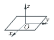
2 Tolerance Zones of Feature Geometric VariationsA feature is the most basic unit which is composed of points, lines and surfaces of parts. And it is a bridge between underlying geometric elements and parts as a carrier of geometric information. The new generation GPS system gives the definition of part features in detail. The definition of features is not the same at different stages from design, manufacturing to inspection, verification according to the new generation GPS system. As shown in Fig. 1, the nominal feature refers to as an ideal cylinder surface without any errors, which is consistent with the designer's imagination. The centerline of the cylinder is defined as nominal derived feature and the distance from any generatrix of cylinder surface to its centerline is the same. The fabricated workpiece constitutes the real integral feature. Workpiece inspection is to determine the shape deviation from nominal geometric features by scanning the actual features using measuring and testing equipment.However, due to the measurement errors, the points recorded by the measuring and testing equipment show great differences from the real surface points. The extracted points from the measurement are composed of the extracted integral feature.During the stage of verification the extracted points need to be evaluated by computer to simulate an ideal cylinder surface based on the given evaluation principle. This simulated cylinder surface makes up the associated feature, and its axis is the associated derived feature.

|
Figure 1 Taxonomy of geometric features(An example of cylinder feature) |
Various types of dimensional and geometrical feature variations have different meanings in actual engineering. The new GPS standards also give the taxonomy of these feature variations. In accordance with the new generation GPS system, the geometrical variations are classified into five categories, i.e., size, shape, orientation, location, and run-out. The size class can control the size variations directly, but cannot control the geometrical errors of the target feature. The form variations only control form deviations of a target feature without any datum. The orientation variations control the angular relations of a target with respect to its datum directly and also control the shape deviations of the target indirectly. The location variations control the location deviations of a target feature from a reference directly. They also indirectly control the orientation and shape deviations of the feature. The run-out class is used to control the straightness, profile, angularity, and other geometrical deviations.
The new generation GPS system also gives the concepts and complementary application of surface model, invariance class, Degree of Invariance (DOI), intrinsic and situation feature etc., to take a massive leap forward for digital control function of geometrical feature from the definition, description, specification to the actual inspection evaluation process. In the new GPS system, the geometries of workpieces are divided into seven types of commonly used which are called seven invariance classes. Seven invariance classes and their DOIs are shown in Table 1.
| Table 1 Seven invariance classes in the new GPS system |


Every feature is one of the seven invariance classes, and each invariance class has its corresponding DOI. If the feature remains unchanged when it rotates around axes x, y, z, or translates along these axes, we call it the DOI of corresponding direction. For instance, a cylindrical feature keep feature invariant when it rotates around axis x and translates along axis x, its DOI is 2.
According to the new GPS standards, a tolerance zone is an area that limits tiny geometric variations of a feature.The regular tolerance zones are constituted of two parallel straight lines or curves, two parallel planes or surfaces, circular zone, two concentric circles, cylindrical zone, two coaxial cylinders, parallelepiped zone, or spherical zone[20], and the complex or irregular domains of the geometric variations are usually 3D tolerance zones. These tolerance zones can be modeled and represented by using the SDT parameters, Table 2 shows several kinds of complex tolerance zones and corresponding torsor matrixes.
| Table 2 Tolerance zones and corresponding torsor matrixes[12] |

3 Modeling Method for Complex Feature Geometric Variations 3.1 The Small Displacements Torsor Concept
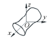
Generally, the variations of any geometrical feature from the nominal position can be represented by using a rotational vector φ around the screw axis and a translational vector ε along this axis.
As shown in Fig. 2, SDT [τ]O consists of the original vector φ and the dual vector εO at a given point O in the Euclidean space.
| $ {\left[ \mathit{\boldsymbol{\tau }} \right]_O} = \left[ {\begin{array}{*{20}{c}} \mathit{\boldsymbol{\varphi }}&{{\mathit{\boldsymbol{\varepsilon }}_O}} \end{array}} \right] = {\left[ {\begin{array}{*{20}{c}} \alpha &u\\ \beta &v\\ \gamma &\omega \end{array}} \right]_O} $ | (1) |

|
Figure 2 The axis equation of torsor |
where εO=ρ×φ+hφ is the dual vector along the screw axis, and h is the pitch of torsor, h=(φ·εO)/(φ·φ).
In Fig. 2, let ρ0 a vector corresponding to a certain point which an axis passes through; and ρ is another vector corresponding to another point which the axis passes through, then the axis equation can be expressed as:
| $ \left( {\mathit{\boldsymbol{\rho }} - {\mathit{\boldsymbol{\rho }}_0}} \right) \times \mathit{\boldsymbol{\varphi }} = 0,\mathit{\boldsymbol{\rho }} \times \mathit{\boldsymbol{\varphi }} = {\mathit{\boldsymbol{\rho }}_0} \times \mathit{\boldsymbol{\varphi }} = {\mathit{\boldsymbol{\varepsilon }}_{\rm{L}}} $ | (2) |
where εL=ρ0×φ is the line moment of the axis relative to the origin of coordinate. And we can see the axis direction and position of torsor can be determined by direction vector φ and line moment εL.
If the origin of coordinate changes, the dual vector will change along with, but the original vector remains the same. Let N a point different from point O in the Euclidean space, as shown in Fig. 3, we have:
| $ {\left[ \mathit{\boldsymbol{\tau }} \right]_N} = \left[ {\begin{array}{*{20}{c}} \mathit{\boldsymbol{\varphi }}&{{\mathit{\boldsymbol{\varepsilon }}_N}} \end{array}} \right] = \left[ {\begin{array}{*{20}{c}} \mathit{\boldsymbol{\varphi }}&{{\mathit{\boldsymbol{\rho }}_N} \times \mathit{\boldsymbol{\varphi }} + h\mathit{\boldsymbol{\varphi }}} \end{array}} \right] $ | (3) |

|
Figure 3 The relocating of torsor |
where φ and εN are a set of dual vectors which compose the torsor [τ]N in N.
Suppose M is another point of Euclidean space, the expression of relative translation vector εM at point M can be derived by using a linearization of the relative rotations.
| $ \begin{array}{l} {\mathit{\boldsymbol{\varepsilon }}_M} = {\mathit{\boldsymbol{\rho }}_M} \times \mathit{\boldsymbol{\varphi }} + h\mathit{\boldsymbol{\varphi }} = \\ \;\;\;\;\left( {{\mathit{\boldsymbol{\rho }}_N} - \overrightarrow {\mathit{\boldsymbol{NM}}} } \right) \times \mathit{\boldsymbol{\varphi }} + h\mathit{\boldsymbol{\varphi }} = \\ \;\;\;\;{\mathit{\boldsymbol{\rho }}_N} \times \mathit{\boldsymbol{\varphi }} - \overrightarrow {\mathit{\boldsymbol{NM}}} \times \mathit{\boldsymbol{\varphi }} + h\mathit{\boldsymbol{\varphi }} = \\ \;\;\;\;{\mathit{\boldsymbol{\varepsilon }}_N} + \mathit{\boldsymbol{\varphi }} \times \overrightarrow {\mathit{\boldsymbol{NM}}} \end{array} $ | (4) |
| $ {\left[ \mathit{\boldsymbol{\tau }} \right]_M} = \left[ {\begin{array}{*{20}{c}} \mathit{\boldsymbol{\varphi }}&{{\mathit{\boldsymbol{\varepsilon }}_M}} \end{array}} \right] = \left[ {\begin{array}{*{20}{c}} \mathit{\boldsymbol{\varphi }}&{{\mathit{\boldsymbol{\varepsilon }}_N} + \mathit{\boldsymbol{\varphi }} \times \overrightarrow {\mathit{\boldsymbol{NM}}} } \end{array}} \right] $ | (5) |
where components of vector
| $ \overrightarrow {\mathit{\boldsymbol{NM}}} = \left[ {\begin{array}{*{20}{c}} {{x_M} - {x_N}}&{{y_M} - {y_N}}&{{z_M} - {z_N}} \end{array}} \right] $ | (6) |
The six intervals of SDT can represent the variation fields of a geometric feature with regard to its nominal position. The SDT is well suited to 3D modeling of complex tolerance zones; it can quantitatively describe the errors of size, shape, orientation, position and run-out of feature variations.
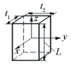
3.2 Modeling of 3D Tolerance Zone Within a ParallelepipedIn this section, we will discuss the tolerance modeling of straightline feature variations. Variation zone is 3D space within a parallelepiped as shown in Fig. 4. This 3D tolerance zone corresponds to straightness, parallelism, perpendicularity, symmetry, position. Origin O of the coordinate system (O, x, y, z) is located at the midpoint of the straightline, and the z direction is consistent with the straightline. The [τ1/0]M characterized the relative position of associated straightline L1 with respect to nominal straightline L0 at any point M of Euclidean space will be:
| $ {\left[ {{\mathit{\boldsymbol{\tau }}_{1/0}}} \right]_M} = \left[ {\begin{array}{*{20}{c}} {{\mathit{\boldsymbol{\varphi }}_{1/0}}}&{{\mathit{\boldsymbol{\varepsilon }}_{1/0,M}}} \end{array}} \right] = \left[ {\begin{array}{*{20}{c}} {{\alpha _{1/0}}}&{{u_{1/0,M}}}\\ {{\beta _{1/0}}}&{{v_{1/0,M}}}\\ 0&0 \end{array}} \right] $ | (7) |

|
Figure 4 3D tolerance zone within a parallelepiped |
The screw [τ1/0]M can transport from point M (xM, yM, zM) to two endpoints A (0, 0, l) and B(0, 0, -l) of the straightline by using Eqs.(4)-(5):
| $ {\left[ {{\mathit{\boldsymbol{\tau }}_{1/0}}} \right]_A} = \left[ {\begin{array}{*{20}{c}} {{\alpha _{1/0}}}&{{u_{1/0,M}} + {\beta _{1/0}}\left( {l - {z_M}} \right)}\\ {{\beta _{1/0}}}&{{v_{1/0,M}} - {\alpha _{1/0}}\left( {l - {z_M}} \right)}\\ 0&{ - {\alpha _{1/0}}{y_M} + {\beta _{1/0}}{x_M}} \end{array}} \right] $ | (8) |
| $ {\left[ {{\mathit{\boldsymbol{\tau }}_{1/0}}} \right]_B} = \left[ {\begin{array}{*{20}{c}} {{\alpha _{1/0}}}&{{u_{1/0,M}} - {\beta _{1/0}}\left( {l + {z_M}} \right)}\\ {{\beta _{1/0}}}&{{v_{1/0,M}} + {\alpha _{1/0}}\left( {l + {z_M}} \right)}\\ 0&{ - {\alpha _{1/0}}{y_M} + {\beta _{1/0}}{x_M}} \end{array}} \right] $ | (9) |
Suppose vector nN is any normal vector of the straightline.
| $ \forall \theta \in \left[ {0,2{\rm{ \mathsf{ π} }}} \right],{\mathit{\boldsymbol{n}}_N}\left[ {\begin{array}{*{20}{c}} {\cos \theta }\\ {\sin \theta }\\ 0 \end{array}} \right] $ | (10) |
In order to ensure that the associated straightline L1 is situated inside the 3D parallelepiped space, the following equations should be satisfied:
| $ \left\{ \begin{array}{l} \left( {k - 1} \right){t_1} \le \left[ {{u_{1/0,M}} + {\beta _{1/0}}\left( {l - {z_M}} \right)} \right]\cos \theta \le k{t_1}\\ \left( {k - 1} \right){t_2} \le \left[ {{v_{1/0,M}} - {\alpha _{1/0}}\left( {l - {z_M}} \right)} \right]\sin \theta \le k{t_2}\\ \left( {k - 1} \right){t_1} \le \left[ {{u_{1/0,M}} - {\beta _{1/0}}\left( {l + {z_M}} \right)} \right]\cos \theta \le k{t_1}\\ \left( {k - 1} \right){t_2} \le \left[ {{v_{1/0,M}} + {\alpha _{1/0}}\left( {l + {z_M}} \right)} \right]\sin \theta \le k{t_2} \end{array} \right. $ | (11) |
where k∈[0, 1].
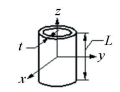
3.3 Modeling of 3D Tolerance Zone Between Coaxial CylindersThis section will discuss the cylindrical surface variations and the tolerance modeling of the corresponding variation zone. As shown in Fig. 5, let S0 a nominal cylindrical surface, the nominal derived feature of the cylindrical surface is axis AB with length 2 m. An orthonormal reference frame is constructed so that x is parallel to the axis of S0 and O is at the midpoint of the nominal derived axis of S0. Suppose [τ1/0]M is the deviation torsor of the associated surface S1 with regard to its nominal surface at point M of Euclidean space which is defined by components β and γ (infinitesimal rotation components around the screw axis) and v and w (infinitesimal translation components along this axis).
| $ {\left[ {{\mathit{\boldsymbol{\tau }}_{1/0}}} \right]_M} = \left[ {\begin{array}{*{20}{c}} {{\mathit{\boldsymbol{\varphi }}_{1/0}}}&{{\mathit{\boldsymbol{\varepsilon }}_{1/0,M}}} \end{array}} \right] = \left[ {\begin{array}{*{20}{c}} 0&0\\ {{\beta _{1/0}}}&{{v_{1/0,M}}}\\ {{\gamma _{1/0}}}&{{w_{1/0,M}}} \end{array}} \right] $ | (12) |

|
Figure 5 3D tolerance zone between coaxial cylinders |
SDT [τ1/0]M can transport from point M to points A and B by using Eqs.(4)-(5):
| $ \begin{array}{*{20}{c}} {{{\left[ {{\mathit{\boldsymbol{\tau }}_{1/0}}} \right]}_A} = \left[ {\begin{array}{*{20}{c}} {{\mathit{\boldsymbol{\varphi }}_{1/0}}}&{{\mathit{\boldsymbol{\varepsilon }}_{1/0,M}} + {\mathit{\boldsymbol{\varphi }}_{1/0}} \times \overrightarrow {\mathit{\boldsymbol{MA}}} } \end{array}} \right] = }\\ {{{\left[ {\begin{array}{*{20}{c}} 0&{ - {\beta _{1/0}}{z_M} + {\gamma _{1/0}}{y_M}}\\ {{\beta _{1/0}}}&{{v_{1/0,M}} + {\gamma _{1/0}}\left( {m - {x_M}} \right)}\\ {{\gamma _{1/0}}}&{{w_{1/0,M}} - {\beta _{1/0}}\left( {m - {x_M}} \right)} \end{array}} \right]}_A}} \end{array} $ | (13) |
| $ \begin{array}{*{20}{c}} {{{\left[ {{\mathit{\boldsymbol{\tau }}_{1/0}}} \right]}_B} = \left[ {\begin{array}{*{20}{c}} {{\mathit{\boldsymbol{\varphi }}_{1/0}}}&{{\mathit{\boldsymbol{\varepsilon }}_{1/0,M}} + {\mathit{\boldsymbol{\varphi }}_{1/0}} \times \overrightarrow {\mathit{\boldsymbol{MB}}} } \end{array}} \right] = }\\ {{{\left[ {\begin{array}{*{20}{c}} 0&{ - {\beta _{1/0}}{z_M} + {\gamma _{1/0}}{y_M}}\\ {{\beta _{1/0}}}&{{v_{1/0,M}} - {\gamma _{1/0}}\left( {m + {x_M}} \right)}\\ {{\gamma _{1/0}}}&{{w_{1/0,M}} + {\beta _{1/0}}\left( {m + {x_M}} \right)} \end{array}} \right]}_B}} \end{array} $ | (14) |
Suppose vector nN is any normal unit vector of S0, nN·x =0, thus we have nN(0, bN, cN). In order to ensure the associated surface S1 is situated inside the region between two coaxial cylinders spaced with a distance t, whose axes are paralleled the nominal derived axis of S0 (see Fig. 5), the variation torsor of the two terminal points A and B on the nominal derived feature of S0 should satisfy the following equation:
| $ \begin{array}{*{20}{c}} {\left( {k - 1} \right)t \le \left[ {{v_{1/0,M}} + {\gamma _{1/0}}\left( {m - {x_M}} \right)} \right] \cdot {b_N} + \left[ {{w_{1/0,M}} - } \right.}\\ {\left. {{\beta _{1/0}}\left( {m + {x_M}} \right)} \right] \cdot {c_N} \le kt} \end{array} $ | (15) |
| $ \begin{array}{*{20}{c}} {\left( {k - 1} \right)t \le \left[ {{v_{1/0,M}} - {\gamma _{1/0}}\left( {m + {x_M}} \right)} \right] \cdot {b_N} + \left[ {{w_{1/0,M}} + } \right.}\\ {\left. {{\beta _{1/0}}\left( {m + {x_M}} \right)} \right] \cdot {c_N} \le kt} \end{array} $ | (16) |
The irregular surface variations and the tolerance modeling of the corresponding variation zone will be discussed in this section. SDT [τ1/0]N represented the relative position of an ideal surface S1 with regard to its nominal surface S0 at a given point N on S0 is composed of infinitesimal rotation vector φ1/0 and infinitesimal translation vector ε1/0, N, the unit vector nN is the normal at point N on S0, as shown in Fig. 6.
| $ {\left[ {{\mathit{\boldsymbol{\tau }}_{1/0}}} \right]_N} = \left[ {\begin{array}{*{20}{c}} {{\mathit{\boldsymbol{\varphi }}_{1/0}}}&{{\mathit{\boldsymbol{\varepsilon }}_{1/0,N}}} \end{array}} \right] = \left[ {\begin{array}{*{20}{c}} {{\alpha _{1/0}}}&{{u_{1/0,N}}}\\ {{\beta _{1/0}}}&{{v_{1/0,N}}}\\ {{\gamma _{1/0}}}&{{w_{1/0,N}}} \end{array}} \right] $ | (17) |

|
Figure 6 3D tolerance zone between equidistant surfaces |
The variation zone of the irregular surface can be set as the space between two equidistant surfaces with a spacing of t. These two equidistant surfaces built by positive and negative offsettings of S0 form a space in which S1 should be located, as shown in Fig. 6. To ensure that the associated surface S1 is located in the spatial region delimited by the two equidistant surfaces, the following equation should be met:
| $ \begin{array}{l} \forall N \in {S_0}\\ \left( {k - 1} \right)t \le {\mathit{\boldsymbol{\varepsilon }}_{1/0,N}} \cdot {\mathit{\boldsymbol{n}}_N} \le kt\;{\rm{with}}\;k \in \left[ {0,1} \right] \end{array} $ | (18) |
where vector nN(aN, b N, c N) is any normal vector of S0, the value of k and t are specified by the designer.
Based on the transport rule of SDT, the relative translation vector ε1/0, M at any point M of Euclidean space can be derived in light of translation vector ε1/0, N and cross product of vector φ1/0 and vector
| $ \left( {k - 1} \right)t \le \left( {{\mathit{\boldsymbol{\varepsilon }}_{1/0,M}} + {\mathit{\boldsymbol{\varphi }}_{1/0}} \times \overrightarrow {\mathit{\boldsymbol{NM}}} } \right) \cdot {\mathit{\boldsymbol{n}}_N} \le kt $ | (19) |
where components of vector
Then, we have the following equation:
| $ \begin{array}{l} \left( {k - 1} \right)t \le \left[ {{u_{1/0,M}} + {\beta _{1/0}}\left( {{z_M} - {z_N}} \right) - {\gamma _{1/0}}\left( {{y_M} - } \right.} \right.\\ \;\;\;\;\;\;\;\;\;\;\;\left. {\left. {{y_N}} \right)} \right]{a_N} + \left[ {{v_{1/0,M}} + {\gamma _{1/0}}\left( {{x_M} - {x_N}} \right) - } \right.\\ \;\;\;\;\;\;\;\;\;\;\;\left. {{\alpha _{1/0}}\left( {{z_M} - {z_N}} \right)} \right]{b_N} + \left[ {{w_{1/0,M}} + {\alpha _{1/0}}\left( {{y_M} - } \right.} \right.\\ \;\;\;\;\;\;\;\;\;\;\;\left. {\left. {{y_N}} \right) - {\beta _{1/0}}\left( {{x_M} - {x_N}} \right)} \right]{c_N} \le kt \end{array} $ | (20) |
From Eq.(20), we can deduce the limits of six components of SDT [τ1/0].
3.5 Modeling of Geometric Feature with Composite TolerancesSome feature variations are constrained by composite dimensional and geometric tolerances. Next, we will discuss the modeling of the plane feature variations with dimensional and geometric tolerances simultaneously as shown in Fig. 7.

|
Figure 7 Plane feature with composite tolerances |
According to the tolerance semantics in the new GPS, the dimensional tolerance zone is non-removable; the parallelism tolerance zone can translate; the flatness tolerance zone can both translate and rotate. The two limit positions of translational motion of parallelism tolerance zone are shown in Fig. 8. The parallelism tolerance zones can only vary within this limit range. Obviously, in order to keep the tolerance semantics of the parallelism tolerance, the variation rangle of the nominal plane will be:
| $ \left\{ \begin{array}{l} - {t_L} \le {\rm{d}}y \le + {t_U}\\ \left| {{\rm{d}}y} \right| \le \frac{{{t_2}}}{2} \end{array} \right. $ | (21) |

|
Figure 8 Two limit variation positions of parallelism tolerance zone |
After having randomly determined the position of parallelism tolerance zone, the result tolerance zone will locate between the parallelism and size tolerance zones. According to the different position of parallelism tolerance zone, there will have three different situations:the first situation is that the result tolerance zone and the parallelism tolerance zone have the same lower boundary, and the result tolerance zone and the size tolerance zone have the same upper boundary; the second one is that the result tolerance zone and the parallelism tolerance zone have the same lower and upper boundaries; the last situation is that the result tolerance zone and the size tolerance zone have the same lower boundary, and the result tolerance zone and the parallelism tolerance zone have the same upper boundary.
Suppose the result tolerance is t3. Then according to the relative positions of flatness tolerance zone and result tolerance zone, SDT [τ1/0]M represented the relative positions of the feature plane with regard to its nominal plane at any point M can be expressed as:
| $ {\left[ {{\mathit{\boldsymbol{\tau }}_{1/0}}} \right]_M} = \left[ {\begin{array}{*{20}{c}} {{\mathit{\boldsymbol{\varphi }}_{1/0}}}&{{\mathit{\boldsymbol{\varepsilon }}_{1/0,M}}} \end{array}} \right] = \left[ {\begin{array}{*{20}{c}} \begin{array}{l} {\alpha _{1/0}}\\ 0\\ {\gamma _{1/0}} \end{array}&\begin{array}{l} 0\\ {v_{1/0,M}}\\ 0 \end{array} \end{array}} \right] $ | (22) |
At any poine N of nominal plane P0 as shown in Fig. 9, the normal vector nN is perpendicular to plane P0 with nN (0, 1, 0). According to the research conclusion above, the following equation ensures that the assigned plane is situated inside the required tolerance zone:
| $ \begin{array}{l} \forall N \in \left( C \right),\left( C \right)\;{\rm{boundary}}\;{\rm{of}}\;{P_0},k \in \left[ {0,1} \right]\\ \;\;\;\left( {k - 1} \right)\left( {{t_1} + {t_3}} \right) \le {v_{1/0,M}} - {\alpha _{1/0}}\left( {{z_N} - {z_M}} \right) + \\ \;\;\;\;\;\;\;\;\;\;\;\;{\gamma _{1/0}}\left( {{x_N} - {x_M}} \right) \le k\left( {{t_1} + {t_3}} \right) \end{array} $ | (23) |

|
Figure 9 Plane feature variation interval range |
4 Illustrative Example
In order to illustrate the application of the presented tolerancing model, a centring pin mechanism used by Ghie et al.[21] is studied. The centring pin mechanism consists of three parts, the detailed drawings of these three parts are shown in Fig. 10. The variation of vertical displacement of the centring pin is functional requirement (FR), which is an important parameter of this assembly necessary to be controlled.

|
Figure 10 A three-part centring pin mechanism(Unit:mm) |
Some key tolerance values labeled in the figure are given in Table 3.
| Table 3 Assigned tolerance values |
To determine the vertical displacement variations of the centring pin (see Fig. 10), some effective feature surfaces associated with the FR of this assembly should be identified. There exist six effective geometric features associated with the FR as shown in Fig. 11.

|
Figure 11 Associated features and local coordinate systems |
These six features are P1, 1 and S1, 2 in part 1, S2, 1 and S2, 2 in part 2, S3, 1 and S3, 2 in part 3, respectively. The notation of an effective feature is composed of two number separated by a ", ", for example S3, 2 signifies surface 2 of part 3. The variations of these features will be represented using presented tolerancing model, then these feature variations can be accumulated to deduce the requested variation value. The local coordinate systems set up on the effective features are also shown in Fig. 11.
The cumulative torsor τ1, 1/3, 1 (the deviation torsor of feature P1, 1 relative to feature S3, 1) can be expressed as:
| $ \begin{array}{l} {\mathit{\boldsymbol{\tau }}_{1,1/3,1}} = {\mathit{\boldsymbol{\tau }}_{1,1/1,2}} + {\mathit{\boldsymbol{\tau }}_{1,2/2,2}} + {\mathit{\boldsymbol{\tau }}_{2,2/2,1}} + {\mathit{\boldsymbol{\tau }}_{2,1/3,2}} + \\ \;\;\;\;\;\;\;{\mathit{\boldsymbol{\tau }}_{3,2/3,1}} \end{array} $ |
where torsor τ2, 1/3, 2 can be eliminated because the contact between surfaces S2, 1 and S3, 2 is assumed perfect, implying that torsor τ2, 1/3, 2 would have no effect on the computation of the functional condition. Then, the cumulative torsor τ1, 1/3, 1 will be:
| $ {\mathit{\boldsymbol{\tau }}_{1,1/3,1}} = {\mathit{\boldsymbol{\tau }}_{1,1/1,2}} + {\mathit{\boldsymbol{\tau }}_{1,2/2,2}} + {\mathit{\boldsymbol{\tau }}_{2,2/2,1}} + {\mathit{\boldsymbol{\tau }}_{3,2/3,1}} $ |
where τ1, 1/1, 2 is the deviation torsor of feature point P1, 1 relative to feature surface S1, 2. τ1, 2/2, 2 is the deviation torsor of feature surface S1, 2 relative to feature surface S2, 2, etc.
It is worth noting that the torsor calculation should take into account the combined effects of the dimensional and geometric tolerances when these tolerances occur on the same geometric feature. The variation ranges of torsor components are listed in Table 4.
| Table 4 Torsors details |
According to the components of these torsors, the result tolerance can be calculated as the cumulative sum of z direction translation components of torsors τ1, 1/1, 2, τ1, 2/2, 2, τ2, 2/2, 1 and τ3, 2/3, 1. As a result the variation of FR in the direction of analysis lies in an interval of [-0.376 5, +0.376 5].
5 ConclusionsA SDT-based method for modeling 3D dimensional and geometrical tolerances is presented in this paper. Firstly, the 3D tolerance domains of feature geometric variations and the concept of SDT are introduced, and the variation deviations between nominal feature and fitting feature are decribed by a set of SDT parameters. And then, the tolerance modeling method of several types of complex or irregular 3D variation regions is studied respectively.At last, the numerical example presented here indicates the effectiveness of the proposed method for modeling dimensional and geometrical tolerances. The proposed modeling method based on the complete and coherent mathematical foundation is easy to carry out in CAT systems, and is compatible with the new generation GPS standards.
| [1] |
Cao Yanlong, Zhang Heng, Mao Jian, et al. Study on tolerance modeling of complex surface. International Journal of Advanced Manufacturing Technology, 2011(53): 1183-1188. ( 0) 0)
|
| [2] |
Chen Hua, Jin Sun, Li Zhimin, et al. A comprehensive study of three dimensional tolerance analysis methods. Computer-Aided Design, 2014, 53(8): 1-13. (0)
|
| [3] |
Khan N S. Generalized Statistical Tolerance Analysis and Three Dimensional Model for Manufacturing Tolerance Transfer in Manufacturing Process Planning. Tempe AZ: Arizona State University, 2011.
(0)
|
| [4] |
Chase K W, Gao J, Magleby S P, et al. Including geometric feature variations in tolerance analysis of mechanical assemblies. ⅡE Transactions, 1996, 28(10): 795-807. DOI:10.1080/15458830.1996.11770732 (0)
|
| [5] |
Marziale M, Polini W. A review of two models for tolerance analysis of an assembly: vector loop and matrix. The International Journal of Advanced Manufacturing Technology, 2009, 43(11-12): 1106-1123. DOI:10.1007/s00170-008-1790-0 (0)
|
| [6] |
Desrochers A, Clément A. A dimensioning and tolerancing assistance model for CAD/CAM systems. The International Journal of Advanced Manufacturing Technology, 1994, 9(6): 352-361. DOI:10.1007/BF01748479 (0)
|
| [7] |
Davidson J K, Mujezinović A, Shah J J. A new mathematical model for geometric tolerances as applied to round faces. Journal of Mechanical Design, 2002, 124(2): 609-621. DOI:10.1115/1.1497362 (0)
|
| [8] |
Mujezinović A, Davidson J K, Shah J J. A new mathematical model for geometric tolerances as applied to polygonal faces. Journal of Mechanical Design, 2004, 126(3): 504-518. DOI:10.1115/1.1701881 (0)
|
| [9] |
Ameta G, Davidson J K, Shah J J. Influence of form on Tolerance-Map-generated frequency distributions for 1D clearance in design. Precision Engineering, 2010, 34(1): 22-27. DOI:10.1016/j.precisioneng.2008.02.002 (0)
|
| [10] |
Ameta G, Davidson J K, Shah J J. Using tolerance-maps to generate frequency distributions of clearance and allocate tolerances for pin-hole assemblies. Journal of Computing and Information Science in Engineering, 2007, 7(4): 347-359. DOI:10.1115/1.2795308 (0)
|
| [11] |
Teissandier D, Couétard Y, Gérard A. A computer aided tolerancing model: Proportioned assembly clearance volume. Computer-Aid Design, 1999, 31(13): 805-817. DOI:10.1016/S0010-4485(99)00055-X (0)
|
| [12] |
Desrochers A, Ghie W, Laperrière L. Application of a unified Jacobian—Torsor model for tolerance analysis. Journal of Computing and Information Science in Engineering, 2003, 3(1): 2-14. DOI:10.1115/1.1573235 (0)
|
| [13] |
Laperrière L, Desrochers A. Modeling assembly quality requirements using Jacobian or screw transforms: a comparison. Proceedings of the IEEE International Symposium on Assembly and Task Planning. Piscataway: IEEE, 2011. 330-336. DOI: 10.1109/ISATP.2001.929044.
http://ieeexplore.ieee.org/xpls/icp.jsp?arnumber=929044
(0)
|
| [14] |
Marziale M, Polini W. A review of two models for tolerance analysis of an assembly: Jacobian and Torsor. International Journal of Computer Integrated Manufacturing, 2011, 24(1): 74-86. DOI:10.1080/0951192X.2010.531286 (0)
|
| [15] |
Bo Chaowang, Yang Zhihong, Wang Linbo, et al. A comparison of tolerance analysis models for assembly. The International Journal of Advanced Manufacturing Technology, 2013, 68(1-4): 739-754. DOI:10.1007/s00170-013-4795-2 (0)
|
| [16] |
Ghie W. Statistical analysis tolerance using Jacobian torsor model based on uncertainty propagation method. International Journal of Multiphysics, 2009, 3(1): 11-30. DOI:10.1260/175095409787924472 (0)
|
| [17] |
Ghie W, Laperrière L, Desrochers A. Statistical tolerance analysis using the unified Jacobian-Torsor model. International Journal of Production Research, 2010, 48(15): 4609-4630. DOI:10.1080/00207540902824982 (0)
|
| [18] |
Zuo Xiaoyan, Li Beizhi, Yang Jianguo, et al. Application of the Jacobian-torsor theory into error propagation analysis for machining processes. The International Journal of Advanced Manufacturing Technology, 2013, 69(5-8): 1557-1568. DOI:10.1007/s00170-013-5088-5 (0)
|
| [19] |
Chen Hua, Jin Sun, Li Zhimin, et al. A modified method of the unified Jacobian-torsor model for tolerance analysis and allocation. International Journal of Precision Engineering and Manufacturing, 2015, 16(8): 1789-1800. DOI:10.1007/s12541-015-0234-7 (0)
|
| [20] |
Khodaygan S, Movahhedy M R, Fomani M S. Tolerance analysis of mechanical assemblies based on modal interval and small degrees of freedom (MI-SDOF) concepts. The International Journal of Advanced Manufacturing Technology, 2010, 50(9-12): 1041-1061. DOI:10.1007/s00170-010-2568-8 (0)
|
| [21] |
Ghie W, Laperrière L, Desrochers A. Re-design of Mechanical Assembly Using the Unified Jacobian-Torsor Model for Tolerance Analysis. In: Davidson J K (ed. ) Models for Computer Aided Tolerancing in Design and Manufacturing. Berlin: Springer, 2007. 95-104.
http://link.springer.com/chapter/10.1007/1-4020-5438-6_11
(0)
|