2. CSR Qindao Sifang Co., Ltd., Qindao 266111, China
Visual object tracking is generally used to identify, locate, and track one or more moving objects over time with a camera, which is one of the core problems in computer vision and applied in many applications, such as intelligent human-computer interaction, security, video surveillance and analysis[1], compression, augmented reality, traffic control, medical imaging[2], video editing[3], et al.It also functions as a core part of scene analysis and behavior recognition.Although visual object tracking has a history for decades and much progress has been achieved in last several years[4-5], the performance of a tracking algorithm is affected by three main factors.The first factor is the appearance changing of the target.The target may endures affine transformation, which cause scale, rotation, and position variation, or the object is composed of several parts which are chained together, or even the object is non-rigid structure or deformable.The second factor is the motion between the camera and object, which may change the orientation of the object over time or abrupt object motion makes the projected trajectory of the object in image complicated.The third factor comes from the environment of the background.The background may be complex and there are may exist some other objects which look like the target.Because of the observation noise, it's hard to recognize the target from the background.Besides the illumination variation, occlusion and other factors, visual object tracking is still a challenging problem and there is no single approach that can successfully handle all scenarios.
Considerable works has been done during the last few decades, Ref.[6] makes an insightful review on this topic.In some case, the target to be tracked can be known in advance, then it is possible to consider much prior knowledge into the design of the tracker.In other case, the designed tracker must be capable of modeling the target appearance on the fly and update the model during the tracking process to account for the target motion, illumination and occlusion.The tracking-by-detection approach[7] formulates the tracking task as a repeated detection over time.Under the framework of tracking-by-detection, the classifiers can be trained online, which provides a natural updating mechanism for adaptive tracking[8-9].
Based on the tracking-by-detection framework, most of the proposed methods are focused on object representation scheme and model updating.For the target representation, it is one of the major component for the tracking algorithm, and many object representation schemes have been proposed.The early works include Lucas and Kanade (LK)[10], raw intensity value based holistic templates have been widely used for tracking[11-12].To better account for appearance changes, subspace-based tracking approaches have been proposed[13-15].In Ref.[15], to account for target appearance variation, a low-dimensional subspace representation is employed and learned incrementally[16].Recently, some sparse representation schemes have been proposed.For example, local sparse representations and collaborative representations have been led in for object tracking[17-18].Zhong et al.[18] had put forward a collaborative tracking algorithm that combined the sparsity-based discriminative classifier with the sparsity-based generative model.These works show some ascendancies of sparse representation in handling the occlusion.To improve run-time performance, a minimal error bounding strategy was proposed[19] to reduce the quantity of ℓ1 minimization problems to be solved.The local binary patterns (LBP)[20] and Haar-like features[21] have also been used to model the tracking object for its appearance.
Recently, many discriminative model-based object tracking methods have been developed, where a binary classifier learns to distinguish the target from the background using online data.Some classifiers, like support vector machine (SVM) [7], structured output SVM[22], ranking SVM[23], boosting[24], semi-boosting[25], and online multi-instance boosting[26], have been adjusted for object tracking.To extract samples effectively for training online classifiers, a number of supervised or semi-supervised methods have been proposed.Grabner et al.[25]devised the update problem to be a semi-supervised task where labeled and unlabeled data were both received by the classifier.By the semi-online boosting algorithm, the model drifting problem can be alleviated.Yu et al.[27] proposed a co-training method for visual tracking, it combines discriminative and generative models.Kalal et al.[28] presented a semi-supervised learning framework to select negative and positive samples for model updating.To make a compromise between the tracking drifting and adaptivity, Stalder et al.[29] integrated semi-supervised classifiers with multiple supervised for tracking.In Ref.[23], the tracking is formulated as a weakly supervised learning problem.
Most of the aforementioned methods are not suitable for long term tracking task, or only currently tested with short term scenarios.They are prone to drifting and weakly in handling out-of-view issues and long-term occlusion.For short-term visual tracking task, the appearance of the target to be tracked does not change greatly, it's the same for the illumination variation.But for the long-term visual tracking task, there are many problems which must be carefully handled.For example, the conflict between plasticity and stability regarding online model update in visual tracking is by no means a trivial thing, and so does the detection of the target when it is out of sight for some time and reappears.Generally speaking, a good long-term visual tracking approach must deal with the illumination variation, scale change, partial occlusions, and background clutter too.All of these factors make the long-term visual tracking very challenging.
There are some papers addressed the long-term tracking problem.For example, to alleviate the stability-plasticity dilemma which is about the online model update, Kalal et al.[30] decomposed the visual tracking problem into three sub-tasks, that is, detection, tracking and learning, where the tracking was formulated as an online learning problem, and the goal was learning an appearance classifier to discriminate the target from the background.In this tracking-by-detection approach, detection and tracking benefit each other, i.e., the results of the tracker provide training data which can be used for updating the detector, meanwhile the detector will re-initialize the tracker when the tracker fails.This cooperative mechanism is demonstrated to work well in long-term tracking task [31-32].A tracker called ALIEN is proposed by Pernici and Bimbo[33-34], which is based on a nearest neighbour classifier, where the classifier tracks using an oriented bounding box, and can handle occlusions well.Ma et al.[35]decomposed the tracking task into two parts, translation estimation and scale estimation of objects, the correlation results between temporal contexts is applied to improve the reliability and accuracy of translation estimation, while an online random fern classifier is trained to re-detect the objects when tracker fails.
The cooperative framework of TLD makes it suitable for long-term visual tracking application, its performance is also confirmed by extensive experiments.Compared with other algorithms, such as Multiple Instance Learning (MIL)[36-37], Co-trained Generative-Discriminative tracking (COGD)[27], Online Random Forrest (ORF)[38-39], more accurate results can be obtained with TLD tracker.Because of this, some further improving works have been conducted based on original TLD algorithm.For instance, the position prediction provided by Kalman filter can greatly decrease the searching range used by the detector[40-44].In Ref.[44], the mean-shift algorithm is used for replacing the media-flow tracker of TLD, and the overall computing load is improved.In Ref.[45], a multiple objects tracking version is extended based on the original single object tracking algorithm.All these works improve the initial TLD algorithm from different aspects.But our extensive experiments show that if the object makes out-of-plane rotation, the media-flow tracker may drift and even fail to track the object, only when the object is re-initialized, the tracker can continue to work.Moreover, the TLD algorithm is not robust against illumination change, and the object rotation.Although with some further improvement, such as optimized C++ implementation, rotation-in-plane tracking, saving and loading learned models, an improved version-TLD2.2 is released[39], as far as we know, there are few of papers discussed about the later issues.
In this paper, we address the robustness improvement of TLD under illumination changing condition.After some initial experiments and comparison, we improve the detector of TLD with the local binary pattern (LBP).LBP method[47] has the advantages such as texture detecting and gray scale invariant, and it is a powerful method for invariant texture classification.To integrate LBP into the tracking-by-detection framework, some modifications of LBP algorithm are made to adapt to the framework of TLD.Kalman filter is used to improve the efficiency.The proposed approach is named as TLD_ULBP and its performance is evaluated with extensive experiments.
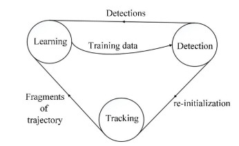
2 Related Works 2.1 Original TLD AlgorithmOriginal TLD algorithm fuses the tracker with detector, and decomposes the visual tracking problem into three sub-tasks, detection, learning and tracking.Every sub-task is completed by a single module, which makes it simple.The block diagram of TLD can be illustrated in Fig. 1[30].
|
Figure 1 Three sub-tasks in TLD framework |
Based on Median-Flow algorithm, the tracker predicts the target position in the coming frame according to the present frame.Lucas-Kanade algorithm is employed by Median-Flow tracker to predict the target motion first, then the matching similarity and the Forward-Back error are calculated.By screening, only about less than half of the feature points will be left.These left feature points will be used to calculate the boundary of targets.The detector will detect all appearances which have been observed so far and can correct the tracker when necessary, which is based on three cascaded classifiers, include patch variance, ensemble classifier and nearest neighborhood (NN) classifier, as showed in Fig. 2.The patch variance filter calculates each pattern's variance, and if the result is less than 50% of the patch selected for tracking, then this pattern is rejected.The ensemble classifier consists of ten basic classifiers, each basic classifier will perform 13 pixel comparisons on the patch and results in a binary code x, which indexes to an array of posteriors Pi(y|x), here y∈(0, 1).The posteriors from individual basic classifiers are averaged, if the average posterior is larger than 50% then the ensemble takes the patch as the target.

|
Figure 2 Three cascaded classifiers of the detector in TLD |
The left patches which are filtered out by variance and ensemble classifier is only about less than about 50%.The nearest neighbor classifier will take these patches as input and calculates two similarities, the conservative and relative similarity, and then choose the patches which relative similarity is greater than a preset threshold as the detector's output.
The learning module in Fig. 1 estimates the detector's errors and corrects it to avoid the errors in future.The object detector is initialized in the very first frame and the detector is updated in the tracking process using the N-expert and the P-expert.P-expert is mainly to find the new appearances of the tracked object.N-expert is mainly used to generate negative training examples.The goal of N-expert is to discover clutter in the background of the environment against which the detector should recognize.
The data processing architecture of the three sub-tasks is illustrated in Fig. 3.

|
Figure 3 Data flow of three sub-tasks in TLD |
2.2 LBP Algorithm
Local binary patterns (LBPs) is one of the most important statistical features which attracts many researchers in recent years[46].The process to get a LBP code can be illustrated in Fig. 4, a neighborhood around each pixel is defined at first, then it exploits the relationship between neighborhood pixels.Each center pixel will be compared with its neighboring pixels, and the LBP code is then obtained by arranging the compared results in proper order.

|
Figure 4 Example of basic LBP operator |
The initial version of the operator uses a 3×3 neighborhood, which labels the neighborhood pixels of the image by threshold the surrounding pixels with the center pixel value.LBP descriptor can be easily extended to different neighborhood size.Generally, a circular shape of neighborhood generally denoted as (P.R) is defined.The number of sampling points in the neighborhood is denoted by P and the radius of circle is R.
For a given center point (xc, yc) in the image, assume its neighborhood point is (xp, yp), it can be obtained by the following result:
xp=xc+Rcos(2πp/P)
yp=yc-Rsin(2πp/P)
Then the LBP label for the center pixel (xc, yc) of image g(xc, yc) is expressed as follows:
| $ LB{P_{P, R}} = \sum\limits_{p = 0}^{p-1} {s(g({x_p}, {y_p})}-g({x_c}, {y_c})){2^p} $ |
Fig. 5 shows an example of different sampling numbers with same radius, all the radiuses are 2, the sample numbers from left to right are 4, 8 and 12 respectively.

|
Figure 5 The extension of LBP descriptor |
The LBPP, R operator can generate 2p different values which correspond to the 2p different binary patterns formed by the P pixels in the neighborhood.As P increases, LBP species is increasing rapidly.To solve the problem, Ojala proposed a dimension reduction method[47], then the new method which named uniform LBP is created.
To define the "uniform" patterns, a uniformity measure U ("pattern") is proposed, which is correspond to the number of spatial transitions (bitwise 0/1 changes) in the "pattern".Uniform pattern is the one which have U value of at most 2.U is defined as Eq (1).
| $ \begin{array}{l} U\left( {LBP} \right) = {\rm{|}}s\left( {{g_{p-1}}-{g_c}} \right)-s\left( {{g_0} - {g_c}} \right)| + \\ \;\;\;\;\;\;\;\;\;\;\;\;\;\sum\limits_{p = 0}^{p - 1} {s({g_p} - {g_c})} - s({g_{p - 1}} - {g_c}) \end{array} $ | (1) |
where gp represents the pixel values of the circularly symmetric neighborhood, and gc is the value of the center pixel.
Obviously LBP has the advantages of representing the local texture feature, which is gray scale and rotation invariance.Because of its advantages, LBP is widely used specially in texture classification.Many extensions of LBP algorithm have lately been proposed, they show good robustness against illumination, rotation, and noise.
2.3 Kalman Filter-based Visual TrackingThe key task of visual tracking is to determine the target position in an image sequence.The tracking algorithm could locate the target anywhere within the image in time.Detecting objects in every frame is like throwing all the information what we have from previous frames and starting all over again.However if only a smaller region of the image is explored, for example, the same size or a little larger as the target region, then the efficiency could be greatly improved.Another reason is that there might be many other similar looking objects in the image.With the help of the prediction, the possibility of wrong detection can be decreased.So Kalman filter can be used to predict the position of target features[48-49].
Basically, Kalman filter composes of twostage processes, that is, prediction stage and measurement update stage.In prediction stage, the current state value is predicted according to the system process model, along with their uncertainties.When the next measurement is available, the predicted state values obtained in first stage are updated using a weighted average rule, the higher the certainty is, more weight is set for the weighted average estimation.The process is recursively run until it's convergent.According to Markov chain rule, it may run in real time with using the current measurements, the previous state value and its uncertainty value, and no more any past information is required.
And the modeling process includes prediction equation and measurement updating.In our case, a linear system and Gaussion noise is assumed, and the state equation of linear system is
x(k)= Ax(k-1)+ W(k-1)
where x(k) denotes the current state, and x(k-1) is the previous state.A denotes the transition matrix which describes the transition from state x(k-1) to x(k). W(k-1) is usually the white Gaussian noise with zero mean and its covariance matrix is Q.
The measurement equation of KF is given by
| $ z\left( \mathit{\boldsymbol{k}} \right) = {\rm{ }}\mathit{\boldsymbol{Hx}}(k) + \mathit{\boldsymbol{V}}(k) $ | (2) |
In Eq.(2), H represents the measurement matrix and V(k) is the white Gaussian noise with zero mean and its covariance matrix is R.
Based on the minimum mean-square error, Kalman filter estimates the state x(k) given the measurements z(1), …, z(k).
The equations used in the recursive procedure are described as follows.
State vector prediction:
| $ \mathit{\boldsymbol{\hat X}}(k|k-1) = \mathit{\boldsymbol{A\hat X}}(k-1|k-1) + \mathit{\boldsymbol{Bu}}(k) $ | (3) |
Minimum mean-square error prediction:
| $ \mathit{\boldsymbol{\hat P}}(k|k-1) = \mathit{\boldsymbol{A\hat P}}(k-1|k-1)\mathit{\boldsymbol{A}}^{\rm{T}} + \mathit{\boldsymbol{Q}} $ |
The gain matrix is defined as:
| $ \begin{array}{l} \mathit{\boldsymbol{K}}(k) = \\ \mathit{\boldsymbol{\hat P}}(k|k- 1){\mathit{\boldsymbol{H}}^T}(k)*{[\mathit{\boldsymbol{R}} + \mathit{\boldsymbol{H}}(k)\mathit{\boldsymbol{\hat P}}(k|k-1){\mathit{\boldsymbol{H}}^{\rm{T}}}(k)]^{ -1}} \end{array} $ |
Then the state vector prediction is
| $ \begin{array}{l} \mathit{\boldsymbol{\hat X}}(k|k) = \\ \mathit{\boldsymbol{A\hat X}}(k|k- 1) + \mathit{\boldsymbol{K}}(k)*[\mathit{\boldsymbol{Z}}(k)-\mathit{\boldsymbol{H}}(k)\mathit{\boldsymbol{\hat X}}(k|k-1)] \end{array} $ |
And minimum mean-square error update as follows:
| $ \mathit{\boldsymbol{\hat P}}(k|k) = [\mathit{\boldsymbol{I}}-\mathit{\boldsymbol{K}}(k)\mathit{\boldsymbol{H}}(k)]\mathit{\boldsymbol{\hat P}}(k|k -1) $ |
Following the TLD framework, we focus on the detection part of TLD here and try to improve it by combining the LBP texture description.As aforementioned in Section 2, the detector of TLD includes three sub-tasks, patch variance, ensemble classifier and nearest neighborhood (NN) classifier, and they work in a cascade mode.After some initial experiments, we found the last detector plays a key role in the detecting part.We can see this from Fig. 6.It shows that, though the image patches left by the variance filter and ensemble classifier are looked like the tracked target, but most of left patches have some certain deviations.Then the key task of the third classifier is to remove or limit the deviation and pick up the best results.Because of the target motion and the illumination changing, the results of the third classifier may still have large deviation, this may causes the drifting and failure in tracking, and it is necessary to improve the whole performance of the detector, so the overall performance of the algorithm can be enhanced.

|
Figure 6 The target and the image patch examples left by the first two classifiers |
Owing to the characteristics of gray scale invariance of LBP algorithm, it can greatly alleviate the effect of illumination variation.The uniform LBP algorithm has lower dimension and good statistical properties, so we try to improve the performance of the third classification of the detector with LBP feature.The third classification-NN classifier is not replaced by, but enhanced by LBP feature.
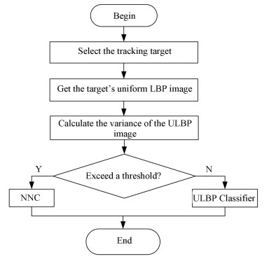
3.1 The Recognition ModuleOur experiments show that when the tracked object has good textures features, the classifier with uniform LBP can work very well.On the other hand, when the texture of the object is not distinctive, the performance of nearest neighbor classifier (NNC) is better.So before the third classifier works, we need to choose the suitable classifier.This is completed by the recognition module.
The recognition module runs in the very initializing phase of TLD_ULBP algorithm.In this module, the tracking target is first selected manually, then the target's uniform LBP (ULBP) image is calculated.The variance of ULBP image is computed to estimate the texture.The experiments show that when the texture variation is less than a threshold, the proposed ULBP classifier can get better output.The flow chart of the recognition module is shown in Fig. 7.
|
Figure 7 Flow chart of the recognition module |
3.2 The Sampling Method
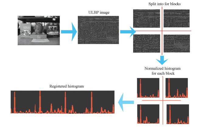
The samples for ULBP classifier are based on ULBP histogram, which should be obtained before running the classifier.Fig. 8 shows the data flow of how to generate the sample.
|
Figure 8 Data generating flow of ULBP samples |
Same as TLD process, the input patches for ULBP are obtained by scanning the window with step size 1.2, horizontal step size is set to 10% of width, vertical step size is set to 10% of height, and the minimal bounding box size is limited to 20 pixels.
Because LBP operator is closely related to location information, if comparing the two uniformed LBP images directly, it may get the wrong result as the non-aligned position.So we use the histogram of uniform LBP image and region segmentation to solve the problem.The ULBP image is separated into multiple sub-regions, LBP features of every sub-region are extracted, then establish uniformed LBP histogram in each sub-region.As a result, each sub-region can be described by a histogram and the entire image consists of a number of statistical histogram.As the tracking object usually occupies a small region of the whole image, so the number of sub-regions is set to four in this paper.The samples of the ULBP classifier are those normalized histogram of ULBP image.Fig. 8 shows data generating flow of the sample.
At the initialization stage of the TLD_ULBP algorithm, when the ULBP classifier is selected as the current third classifier, then by calculating the ULBP histogram of the patches, the positive sample is selected as the patch which is most likely to the tracked target.The negative samples are selected among the patches that have the largest difference with the tracked target.Fig. 9 shows the histogram difference between the positive sample and negative sample.

|
Figure 9 An example of the histogram of ULBP sample |
3.3 The ULBP Classifier
The ULBP classifier is dependent on ULBP histogram.The sample is defined as the normalized uniform LBP histogram.To compare the samples, the measurement of relatively similarity should be defined first.For the comparison of two histograms, the method like Intersection, correlation, Bhattacharyya distance and Chi-Square may be used.Here, the normalized correlation coefficient is employed, which is defined as:
| $ d({\mathit{\boldsymbol{H}}_1}, {\mathit{\boldsymbol{H}}_2}) = \frac{{\sum\nolimits_{\rm{I}} {({\mathit{\boldsymbol{H}}_1}\left( \mathit{\boldsymbol{I}} \right)-{{\mathit{\boldsymbol{\bar H}}}_1})} ({\mathit{\boldsymbol{H}}_2}\left( \mathit{\boldsymbol{I}} \right)-{{\mathit{\boldsymbol{\bar H}}}_2})}}{{\sqrt {\sum\nolimits_{\rm{I}} {{{({\mathit{\boldsymbol{H}}_1}\left( \mathit{\boldsymbol{I}} \right)-{{\mathit{\boldsymbol{\bar H}}}_1})}^2}} {{\sum\nolimits_{\rm{I}} {({\mathit{\boldsymbol{H}}_2}\left( \mathit{\boldsymbol{I}} \right) - {{\mathit{\boldsymbol{\bar H}}}_2})} }^2}} }} $ | (4) |
where
| $ {{\mathit{\boldsymbol{\bar H}}}_K} = \frac{1}{N}\sum\limits_\mathit{\boldsymbol{J}} {{\mathit{\boldsymbol{H}}_\mathit{\boldsymbol{K}}}\left( \mathit{\boldsymbol{J}} \right)} {\rm{ }} $ | (5) |
where N denotes the number of histogram bins, H1 and H2 denote the histograms to be compared, d(.) refers to the correlation coefficient, it is ranged from 0 to 1.When d is equal to 1, that means the two compared histograms are exactly the same.The smaller this value is, the larger of the difference between the two compared histograms will be.A sample is taken as the detected object when d>θ_NN, θ_NN is set to 0.68 in the experiments of this paper, which is selected empirically.
3.4 TrainingIf the target is detected successfully by the ULBP classifier, then the results is used as the input of the P-N learning part.Because we improved the detector in the proposed TLD_ULBP approach, and P-N learning module is necessary to make the correspondent modification.
The samples which have passed the previous two classifiers of the TLD_ULBP detector will be marked as negative samples if its overlap ratios with target are less than 80%.The positive sample is taken as the present target, the normalized ULBP histogram of the sample is provided as the input of P-N learning part.P-N Learning part in TLD is mainly used to correct the error classification.Using Eqs.(4) and (5), the correlation coefficients among the current negative and positive samples with the samples stored in training dataset are calculated.If the correlation coefficient of positive sample is smaller than a threshold, then it indicates that the current output by the classifier is incorrect, then this patch will be put to the dataset for positive sample.Or it will be put to the dataset for negative sample.
3.5 Experiments1) Experiments about illumination changing.
We tested the proposed method with the illumination changing videos.Table 1 shows the properties of these videos.Table 2 presents the performance evaluated with precision/recall/F-measure.
| Table 1 The properties of the test video sequences |
| Table 2 The performance comparison between TLD and TLD_ULBP |
In Table 1, IV indicates the illumination variation, the video marked with IV will mean the illumination especially in the target region is changed significantly.SV represents the scale variation, if the video marked with SV, that means the ratio of the bounding box size between the current frame and the first frame is beyond the range ts, ts>1(ts=2).OCC denotes occlusion, which means the target in the video is partially or fully occluded.MB refers to motion blur, it is usually caused by the motion of camera or target.IPR is the abbreviation for In-Plane Rotation.OPR is the abbreviation for Out-of-Plane Rotation.
For each video sequence, the results with Precision/recall/F-measure index are provided in Table 2.The results in the table show that TLD_ULBP algorithm is outperformed against the original TLD algorithm.
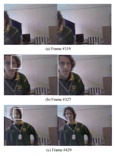
Fig. 10 presents some more details of the experiments.In the figure, the results of the TLD_ULBP method are presented on the left column, the results of the original TLD algorithm is presented on the right column.The white box indicates the final results of the tracker, and the green points inside the white box refer to the feature points of the tracker.If there exists no bounding box, it will mean that the tracking algorithm fails to work in this case.
|
Figure 10 Some more detail comparison between TLD_LBP and TLD(Left column-TLD_LBP, right column-TLD) |
As illustrated in Fig. 10, for frame 327, there is only a white box for TLD_LBP, that means the tracker fails to track the object, however the detector can still detect out the target.There is no white box shown in the right column, it means the detector of the original TLD algorithm fails.
2) Experiments with the standard ten video clips.
We made a performance comparison between the proposed TLD_ULBP and TLD algorithm with the standard ten video sequences that have been extensively used in other literatures.As mentioned above, for the proposed TLD_ULBP algorithm, when the tracked object has rich texture, the ULBP classifier will be selected, or the nearest neighbor classifier will be employed.If the results for a video is good both for the original TLD and the proposed TLD_ULBP algorithm, then it will not be presented in this section.For example, both TLD_ULBP and TLD can obtain good results with the video sequence "David".The results here show that the proposed TLD_ULBP algorithm is outperformed against TLD algorithm for other videos in the dataset.
Table 3 presents the properties of these video sequences, Table 4 shows the experiment results.In Table 4, it shows that the proposed TLD_ULBP can work well and outperform against TLD algorithm except for boy and human 2.For these two video sequences, the performance of TLD_ULBP is very closed to TLD algorithm.
| Table 3 The properties of the video sequences for the experiments |
| Table 4 The performance comparison between TLD and the proposed TLD_LBP |
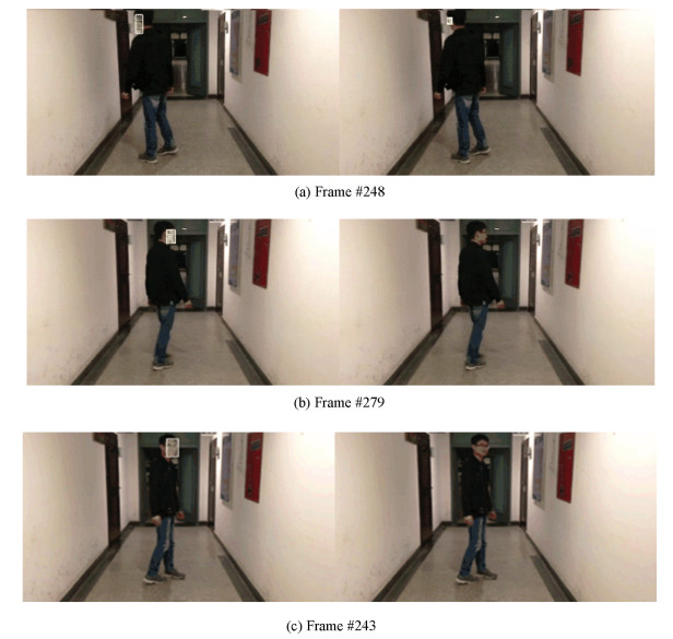
Fig. 11 shows another experiment results with a video sequence recorded by ourselves.As in Fig. 10, the results of the proposed TLD_ULBP are presented on the left column, and the results of TLD algorithm are presented on the right column.When the student turned around, the original TLD failed to track his face.However, the TLD_ULBP algorithm can work well in this case.Fig. 12 shows some snapshots picked from the video clips, it is obvious the proposed TLD_ULBP can work well.
|
Figure 11 Experiment with face tracking(Left column is the results of TLD_ULBP, the right column is the results of the TLD) |

|
Figure 12 The snapshot of the result |
4 Applying Kalman Filter to TLD_ULBP
To improve the efficiency of TLD_ULBP, KF is employed to predict the tracked target position.The state vector is defined as [x, y, w, h, Vx, Vy]T, (x, y) is the centre position of the tracked object, (w, h) denotes the bounding box size of target, and (Vx, Vy) is the velocity of tracking object.Because the time interval of adjacent frames is very short, so a constant motion model is used.The transition matrix A in Eq.(3) is defined as:
| $ \mathit{\boldsymbol{A = }}\left[{\begin{array}{*{20}{l}} 1&0&0&0&t&0\\ 0&1&0&0&0&t\\ 0&0&1&0&0&0\\ 0&0&0&1&0&0\\ 0&0&0&0&1&0\\ 0&0&0&0&0&1 \end{array}} \right] $ |
where t is the time interval of adjacent frames of the video input.
Because the tracking result of TLD_ULBP algorithm has high reliability, so it will be used as the update value of measurement vector.So the measurement vector defined as z =[x, y, Vx, Vy]Tand the matrix H is defined as:
| $ \mathit{\boldsymbol{H = }}\left[{\begin{array}{*{20}{c}} 1&0&0&0\\ 0&1&0&0\\ 0&0&1&0\\ 0&0&0&1 \end{array}} \right] $ |
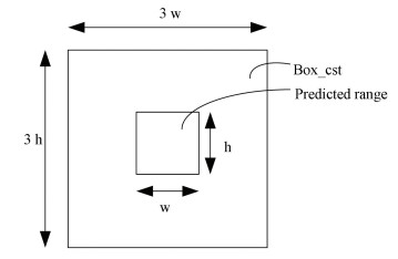
According to the predictive value of Kalman filter, we can get the position and bounding box size of candidate tracking target and then the uniform LBP histogram corresponding to the bounding box size is calculated.An unlabeled sample is generated.Comparing it with the negative and positive sample database, a relatively similarity measurement will be computed.If the relatively similarity is greater than the preset threshold (0.63), the predictive value will be marked as "having a certain credibility".If the tracker successfully tracked the target, at the meantime, the distance between the two parts smaller than a threshold dT, then mark the predictive value as "basic right".By averaging the two boxes, and increasing the obtained box size three times, we can get a box named as "box_cst", which will be used as the detector's searching area, as shown in Fig. 13.
|
Figure 13 Schematic diagram of searching range |
Before sending the samples to the detector, they need to be located within the constrained box, if they are within constraint box, they will be sent to the first classifier, or they will be discarded.By doing this, most of the unlabeled samples can be filtered out.This saves a lot of time in the stage of detector.To be brief, the version with KF optimization of TLD_ULBP is named as TLD_ULKF.
4.1 Experiments on Predicting OptimizationTo compare the efficiency between TLD_ULBP and TLD_ULKF, all the software are running on a computer with windows 7 OS, 64-bit CPU:Intel(R) core i5, 3.00 GHz, memory size is 4 GB, the algorithms are implemented under VS2012 and Opencv2.4.9.
The running time is computed as follows:
For TLD_ULKF:Tulk=Tdec+Tkf;
For TLD_ULBP:Tulbp=Tdec.
Tdec is the time of detector and Tkf is the running time of Kalman filter; The experiment result on video "doll" is shown in Fig. 14.From this figure, we can see that in most of the time, TLD_ULKF runs faster than TLD_ULBP.

|
Figure 14 The running time comparison between TLD_ULBP and TLD_ULKF algorithm |
4.2 Experiments on Accuracy Improvement
Besides the time saving, there is another effect caused by Kalman filter prediction, which is the center point drifting of the target.It is related to the accuracy of the tracking results.
To make the comparison, we first define a center offset as the metric measurement based on Enclidean distance,
| $ {d_o} = \sqrt {{{({x_r}-{x_e})}^2} + {{({y_r}-{y_e})}^2}} $ |
where (xr, yr) is the reference value of the center point, and (xe, ye) is the coordinate of the tracking result.
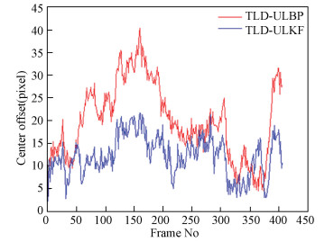
Fig. 15 shows the distance curve between TLD_ULBP and TLD_ULKF algorithm with video "fleetface".The red curve represents the centre offset of TLD_ULBP algorithm, and blue one is the centre offset of TLD_ULKF algorithm.It is obvious that the algorithm TLD_ULKF have better overall performance than TLD_ULBP algorithm.
|
Figure 15 The center offset comparison results for the video "fleetface" |
Table 5 show the result of time cost comparison between TLD_ULBP and TLD_ULKF algorithm with 13 video sequences.If it fails to tracking the object, the tracking result is set to be (0, 0) (generally the centre of the tracked object cannot be located at this point), and
| Table 5 The centre offset comparison result between TLD_ULBP and TLD_ULKF |
In Table 5 we can see that, in addition to video 2 and video 4, the other 11 videos have lower center offset in TLD_ULKF algorithm, this indicates that by integrating the Kalman filter with the TLD_ULBP algorithm, the overall performance of efficiency and accuracy can be improved.
5 Discussion and ConclusionsIn this paper, motivated by the high performance of TLD algorithm for longterm tracking, to further improve its robustness and accuracy under illumination changing, we first integrate LBP feature-based classifier (ULBP) with nearest neighbor (NN) classifier, and a recognition module is well designed to select the suitable one between the ULBP classifier and NN classifier.The ULBP classifier is discussed in detail.Extensive evaluation experiments confirm that the TLD_ULBP can work better than TLD algorithm.To further improve the efficiency of the TLD_ULBP algorithm, we apply the Kalman filter to TLD_ULBP.The experiments confirm that not only the efficiency of the proposed algorithm is improved, but the accuracy is increased too.
For a robust long-term tracking, neither detection nor tracking can solve the tracking tasks independently, and the tracking-by-detection approach provides a novel framework.Our works show that there is still potential improvements space for increasing the performance of TLD.Currently, we have done some initial works on the performance improvement.How the LBP-based classifier affects the drifting of long-term tracking will be explored in the future.We will further improve the efficiency of the proposed method and put it into real-time applications with hardware-limited mobile platform.
| [1] |
Matusek F, Sutor S, Kraus K, et al. NIVSS: A nearly indestructible video surveillance system. Proceeding of the 3rd International Conference on Internet Monitoring and Protection. Washington DC: IEEE Computer Society, 2008, 98-102.
( 0) 0)
|
| [2] |
Mountney P, Stoyanov D, Yang G Z. Three-dimensional tissue deformation recovery and tracking. IEEE Signal Processing Magazine, 2010, 27(4): 14-24. DOI:10.1109/MSP.2010.936728 ( 0) 0)
|
| [3] |
Mihaylova L, Brasnett P, Canagarajan N, et al. Object tracking by particle filtering techniques in video sequences. In: Advances and Challenges in Multisensor Data and Information. NATO Security Through Science Series, 8. Amsterdam: IOS Press, 2007. 260-268.
( 0) 0)
|
| [4] |
Yang H, Shao L, Zheng F, et al. Recent advancesand trends in visual tracking: A review. Neurocomputing, 2011, 74(18): 3823-3831. DOI:10.1016/j.neucom.2011.07.024 ( 0) 0)
|
| [5] |
Smeulders A W M, Chu D M, Cucchiara R, et al. Visual tracking: An experimental survey. IEEE Transaction on Pattern Anal. Mach. Intell., 2014, 36(7): 1442-1468. DOI:10.1109/TPAMI.2013.230 ( 0) 0)
|
| [6] |
Yilmaz A, Javed O, Shah M. Object tracking: A survey. ACM Computing Surveys, 2006, 38(4): 81-93. ( 0) 0)
|
| [7] |
Avidan S. Support vector tracking. IEEE Transactions on Pattern Analysis and Machine Intelligence, 2004, 26(8): 1064-1072. DOI:10.1109/TPAMI.2004.53 ( 0) 0)
|
| [8] |
Grabner H, Grabner M, Bischof H. Real-time tracking via online boosting. Proceedings of the British Machine Vision Conference, 2006, 47-56. DOI:10.5244/C.20.6 ( 0) 0)
|
| [9] |
Saffari A, Godec M, Pock T, et al. Online multi-class LPBoost. 2010 IEEE Conference on Computer Vision and Pattern Recognition (CVPR). Piscataway:IEEE, 2010, 3570-3577. DOI:10.1109/CVPR.2010.5539937 ( 0) 0)
|
| [10] |
Lucas B D, Kanade T. An iterative image registration technique with an application to stereo vision. Proceedings of Imaging Understanding Workshop, 1981, 121-130. ( 0) 0)
|
| [11] |
Matthews I, Ishikawa T, Baker S. The template update problem. IEEE Transactions on Pattern Analysis and Machine Intelligence, 2004, 26(6): 810-815. DOI:10.1109/TPAMI.2004.16 ( 0) 0)
|
| [12] |
Alt N, Hinterstoisser S, Navab N. Rapid selection of reliable templates for visual tracking. 2010 IEEE Conference on Computer Vision and Pattern Recognition. Piscataway: IEEE, 2010, 1355-1362. DOI:10.1109/CVPR.2010.5539812
( 0) 0)
|
| [13] |
Hager G D, Belhumeur P N. Efficient region tracking with parametric models of geometry and illumination. IEEE Transactions on Pattern Analysis and Machine Intelligence, 1998, 20(10): 1025-1039. DOI:10.1109/34.722606 ( 0) 0)
|
| [14] |
Black M J, Jepson A D. Eigentracking: Robust matching and tracking of articulated objects using a view-based representation. International Journal of Computer Vision, 1998, 26(1): 63-84. DOI:10.1023/A:1007939232436 ( 0) 0)
|
| [15] |
Ross D A, Lim J, Lin R-S, et al. Incremental learning for robust visual tracking. International Journal of Computer Vision, 2008, 77(1-3): 125-141. DOI:10.1007/s11263-007-0075-7 ( 0) 0)
|
| [16] |
Isard M, Blake A. CONDENSATION—Conditional density propagation for visual tracking. International Journal of Computer Vision, 1998, 29(1): 5-28. DOI:10.1023/A:1008078328650 ( 0) 0)
|
| [17] |
Zhang T, Ghanem B, Liu S, et al. Robust visual tracking via multi-task sparse learning. IEEE Conference on Computer Vision and Pattern Recognition. Piscataway: IEEE, 2012, 2042-2049.
( 0) 0)
|
| [18] |
Zhong W, Lu H, Yang M H. Robust object tracking via sparse collaborative appearance model. IEEE Transactions on Image Processing, 2014, 23(5): 2356-2368. DOI:10.1109/TIP.2014.2313227 ( 0) 0)
|
| [19] |
Mei X, Ling H, Wu Y, et al. Minimum error bounded efficient L1 tracker with occlusion detection. Computer Vision and Pattern Recognition, IEEE, 2011. ( 0) 0)
|
| [20] |
Ojala T, Pietikainen M, Maenpaa T. Multiresolution grayscale and rotation invariant texture classification with local binary patterns. IEEE Transaction on Pattern Analysis and Machine Intelligence, 2002, 24(7): 971-987. DOI:10.1109/TPAMI.2002.1017623 ( 0) 0)
|
| [21] |
Viola P, Jones M J. Robust real-time face detection. International Journal of Computer Vision, 2004, 57(2): 137-154. DOI:10.1023/B:VISI.0000013087.49260.fb ( 0) 0)
|
| [22] |
Hare S, Saffari A, Torr P H S. Struck: Structured output tracking with kernels. Piscataway: IEEE, 2011, 263-270. DOI:10.1109/ICCV.2011.6126251
( 0) 0)
|
| [23] |
Bai Y, Tang M. Robust tracking via weakly supervised ranking SVM. 2012 IEEE Conference on Computer Vision and Pattern Recognition, 2012, 1854-1861. DOI:10.1109/CVPR.2012.6247884 ( 0) 0)
|
| [24] |
Grabner H, Grabner M, Bischof H. Real-time tracking via on-line boosting. Proceedings of the British Machine Conference. Edinburgh, 2006, 47-56. DOI:10.5244/C.20.6 ( 0) 0)
|
| [25] |
Grabner H, Leistner C, Bischof H. Semi-supervised on-line boosting for robust tracking. European Conference on Computer Vision. ECCV 2008: Computer Vision-ECCV 2008, 2008, 234-247. DOI:10.1007/978-3-540-88682-2_19 ( 0) 0)
|
| [26] |
Babenko B, Yang M-H, Belongie S. Robust object tracking with online multiple instance learning. IEEE Transactions on Pattern Analysis and Machine Intelligence, 2011, 33(8): 1619-1632. DOI:10.1109/TPAMI.2010.226 ( 0) 0)
|
| [27] |
Yu Q, Dinh T B, Medioni G. Online tracking and reacquisition using co-trained generative and discriminative trackers. European Conference on Computer Vision, ECCV 2008: Computer Vision-ECCV 2008, 2008, 678-691. DOI:10.1007/978-3-540-88688-4_50 ( 0) 0)
|
| [28] |
Kalal Z, Matas J, Mikolajczyk K. P-N learning: Bootstrapping binary classifiers by structural constraints. Computer Vision and Pattern Recognition. Piscataway: IEEE, 2010. DOI:10.1109/CVPR.2010.5540231
( 0) 0)
|
| [29] |
Stalder S, Grabner H, van Gool L. Beyond semi-supervised tracking: Tracking should be as simple as detection, but not simpler than recognition. 2009 IEEE 12th International Conference on Computer Vision Workshops (ICCV Workshops). Piscataway: IEEE, 2009, 1409-1416. DOI:10.1109/ICCVW.2009.5457445
( 0) 0)
|
| [30] |
Kalal Z, Mikolajczyk K, Matas J. Tracking-Learning-Detection. IEEE Transactions on Pattern Analysis and Machine Intelligence, 2012, 34(7): 1409-1422. DOI:10.1109/TPAMI.2011.239 ( 0) 0)
|
| [31] |
Supancic J S, Ramanan D. Self-paced learning for long-term tracking. 2013 IEEE Conference on Computer Vision and Pattern Recognition, 2013, 9(4): 2379-2386. DOI:10.1109/CVPR.2013.308 ( 0) 0)
|
| [32] |
Hua Y, Alahari K, Schmid C. Occlusion and motion reasoning for long-term tracking. In Proceedings of the European Conference on Computer Vision, 2014, 172-187. DOI:10.1007/978-3-319-10599-4_12 ( 0) 0)
|
| [33] |
Pernici F. Facehugger: The ALIEN tracker applied to faces. In Proceedings of the European Conference on Computer Vision, 2012, 597-601. DOI:10.1007/978-3-642-33885-4_61 ( 0) 0)
|
| [34] |
Pernici F, Bimbo A D. Object tracking by oversampling local features. IEEE Transactions on Pattern Analysis and Machine Intelligence, 2014, 36(12): 2538-2551. DOI:10.1109/TPAMI.2013.250 ( 0) 0)
|
| [35] |
Ma C, Yang X K, Zhang C Y, et al. Long-term correlation tracking. 2015 IEEE Conference on Computer Vision and Pattern Recognition. Piscataway:IEEE, 2015, 5388-5396. DOI:10.1109/CVPR.2015.7299177 ( 0) 0)
|
| [36] |
Babenko B, Yang M-H, Belongie S. Visual tracking with online multiple instance learning. Computer Vision and Pattern Recognition, 2010, 983-990. ( 0) 0)
|
| [37] |
Zhang K H, Song H H. Real-time visual tracking via online weighted multiple instance learning. Pattern Recognition, 2013, 46(1): 397-411. DOI:10.1016/j.patcog.2012.07.013 ( 0) 0)
|
| [38] |
Leistner C, Godec M, Saffari A, et al. Online multi-view forests for tracking. Joint Pattern Recognition Symposium, 2010, 493-502. DOI:10.1007/978-3-642-15986-2_50 ( 0) 0)
|
| [39] |
Zdenek Kalal. TLD Vision. http://www.tldvision.com/, 2016-12-27.
( 0) 0)
|
| [40] |
Zhou Xin, Qian Qiumeng, Ye Yongqiang, et al. Improved TLD visual target tracking algorithm. Journal of Image and Graphics, 2013, 18(9): 1115-1123. DOI:10.11834/jiq.20130908.(inChinese) ( 0) 0)
|
| [41] |
Teng F, Liu Q, Zhu L, et al. Robust inland waterway ship tracking via hybrid TLD and Kalman filter. Advanced Materials Research, 2014, 1037: 373-377. DOI:10.4028/www.scientific.net/AMR.1037.373 ( 0) 0)
|
| [42] |
Jiang Bo. Research on TLD Algorithm Based on Kalman Filter. Xian: Xidian University, 2013. (in Chinese)
( 0) 0)
|
| [43] |
Zhang Shuailing. Research on Video Target Tracking Algorithm Based on TLD. Xian: Xidian University, 2014. (in Chinese)
( 0) 0)
|
| [44] |
Xiao Q G, Ye Q W, Zhou Y, et al. Long-term video tracking algorithm of optimized TLD based on mean-shift. Application Research of Computer, 2015, 32(3): 925-928. DOI:10.3969/j.issn.1001-3695.2015.03.066.(inChinese) ( 0) 0)
|
| [45] |
Yu G Z. Research on Multi-target Tracking Based on TLD Algorithm. Xiamen: Xiamen University, 2012. (in Chinese)
( 0) 0)
|
| [46] |
Huang D, Shan C F, Ardabilian M, et al. Local binary patterns and its application to facial image analysis: A survey. IEEE Transactions on Systems, Man, and Cybernetics-part C: Applications and Reviews, 2011, 41(6): 765-781. DOI:10.1109/TSMCC.2011.2118750 ( 0) 0)
|
| [47] |
Ojala T, Pietikäine M, Mäenpää T. Multiresolution gray scale and rotation invariant texture classification with local binary patterns. IEEE Transactions on Pattern Analysis and Machine Intelligence, 2002, 24(7): 971-987. DOI:10.1007/3-540-45054-8_27 ( 0) 0)
|
| [48] |
Liu J, Sun H, Yang H, et al. CamShift based on multi-feature fusion and Kalman prediction for real-time visual tracking. Information Technology Journal, 2014, 13(1): 159-164. DOI:10.3923/itj.2014.159.164 ( 0) 0)
|
| [49] |
Karavasilis V, Nikou C, Likas A. Visual tracking by adaptive Kalman filtering and mean shift. . Artificial Intelligence: Theories, Models and Applications. Springer Berlin Heidelberg, 2010, 153-162. DOI:10.1007/978-3-642-12842-4_19
( 0) 0)
|
 2018, Vol. 25


