 2018, Vol. 25


2. College of Engineering, The University of Iowa, Iowa City, IA 52242, USA
Fault study of rotor systems is one of key focus points in rotor dynamics, appealing to the concern of a series of researchers in different areas. The common faults include pedestal looseness fault[1-3], rotor-stator rub-impact fault[4-8], crack fault[9-12], ball bearing fault[13-15], misalignment fault[16-17], coupling fault[18-19], etc. The research on pedestal looseness is relatively less than that on other faults in the rotor system now. A majority of researchers studied looseness based on the bearing pedestal looseness of sole end or combining with the rub-impact fault[1-3, 18-19]. But looseness may lead to looseness at the other end in actual operating condition, so pedestal looseness at both ends plays a key role in the fault study of rotor systems.
As is known to all, most rotor-bearing systems are multi-DOF and complex. The qualitative analysis cannot provide comprehensive guidance to multi-DOF systems and the corresponding calculation quantities are extremely huge. The original systems for dimension reduction should be studied.There are many dimension reduction methods, such as center manifold method, POD method, Galerkin method, inertial manifold method, etc. Rega and Steindl[20-21] summarized these methods in their research about nonlinear dynamics.Many researchers used POD method to study dynamic behaviors of multi-DOF actual rotor bearing systems. The POD method is an efficient method to obtain reduced models to replace the original ones [22].The nonlinear POD method was used to study the multi-DOF rotor-bearing system, and the efficiency of the dimension reduction method was verified[23]. The TPOD method was proposed via combining the POD method with approximately inertial manifold theory, the TPOD method was used in rotor system supported by liquid-film bearings, and the relative order reduction error was less than 5% [24]. The method was also used to simplify the original rotor system supported by ball bearings to a reduced one, stability of the reduced model was analyzed [25].
The DOF number of the reduced model is a substantial part during the order reduction process. The proper orthogonal value (POV) of the correlation matrix reflects the energy of the related proper orthogonal mode (POM). The percentage of the largest POVs related to the dominant proper orthogonal modes (POMs) occupying all non-negative eigenvalues can obtain the appropriate DOF of the reduced model[26-27]. The POM energy stands for the case of the dynamics behaviors of the reduced system occupies the original one. The characters of the simplified system occupy more as the energy increases. As usual, the number of DOF is considered to be appropriate when the energy is higher than 99%[28]. Lu applied the POM energy method to describe the physical interpretation of the TPOD method in rotor-bearing system [25, 29], and the first two order POM energy contains almost 99.99% of the original 7-DOFs and 15-DOFs rotor systems. The first order POM reserves the primary energy of the rotor system supported by nonlinear stiffness via the confirmation of POM energy method[30].
The aim of this paper is to discuss pedestal looseness behaviors of the original and simplified rotor systems.Pedestal looseness behavior is analyzed by comparing the fault-free model with the looseness faults models. The effects of initial values are analyzed.The TPOD method is used to simplify the high-dimensional systems to the 6-DOFs ones. The efficiency of the dimension reduction method is validated in comparison to bifurcation and amplitude-frequency behaviors.
2 Dynamical System Model of Rotor SystemIn this section, rotor models supported by liquid-film bearings with one end and both ends pedestal looseness are respectively established. The 23-DOFs rotor model with one end looseness was applied in Ref. [24] by the author. For convenience, we only provide the dynamical equation of 24-DOFs rotor model with both ends looseness.
Figs. 1-3 show the 22-DOFs, 23-DOFs and 24-DOFs rotor models respectively, the assumed conditions and the system parameters are the same as those in Ref. [24]. The corresponding assumption conditions are the same as those in Ref. [29]. Y12 and Y13 are the pedestal displacements at both ends, the expression is as follows:
| $ {k_{SL}} = \left\{ {\begin{array}{*{20}{l}} {{k_{SL1}},{Y_{12}} > {\delta _1}}\\ {0,\;\;\;\;0 \le {Y_{12}} \le {\delta _1}}\\ {{k_{SL2}},{Y_{12}} < 0} \end{array}} \right. $ |
| $ {c_{SL}} = \left\{ \begin{array}{l} {c_{SL1}},{Y_{12}} > {\delta _1}\\ 0,\;\;\;\;0 \le {Y_{12}} \le {\delta _1}\\ {k_{SL2}},{Y_{12}} < 0 \end{array} \right. $ |
| $ {k_{SR}} = \left\{ \begin{array}{l} {k_{SR1}},{Y_{13}} > {\delta _2}\\ 0,\;\;\;\;0 \le {Y_{13}} \le {\delta _2}\\ {k_{SR2}},{Y_{13}} < 0 \end{array} \right. $ |
| $ {c_{SL}} = \left\{ \begin{array}{l} {c_{SR1}},{Y_{13}} > {\delta _2}\\ 0,\;\;\;\;0 \le {Y_{13}} \le {\delta _2}\\ {c_{SR2}},{Y_{13}} < 0 \end{array} \right. $ |

|
Figure 1 22-DOFs fault free model |

|
Figure 2 23-DOFs pedestal looseness model at left end |

|
Figure 3 24-DOFs pedestal looseness model at both ends |
In Fig. 3, the motion differential equations can be obtained and we can also get the dimensionless form, see details in formulas (1) and (2).
| $ \mathit{\boldsymbol{\tilde M\ddot {\tilde Z}}} + \mathit{\boldsymbol{\tilde C\dot {\tilde Z}}} + \mathit{\boldsymbol{\tilde K\tilde Z}} = \mathit{\boldsymbol{\tilde F}} $ | (1) |
In Eq.(3),
| $ \mathit{\boldsymbol{\tilde Z}} = {\left( {\begin{array}{*{20}{c}} {{X_1}}&{{Y_1} \cdots {Y_{11}}}&{{Y_{11}}}&{{Y_{12}}}&{{Y_{13}}} \end{array}} \right)^{\rm{T}}} $ |
| $ \mathit{\boldsymbol{\tilde M}} = {\rm{diag}}\left( {{m_1},{m_1}, \cdots ,{m_{11}},{m_{11}},{m_{12}},{m_{13}}} \right) $ |
| $ \mathit{\boldsymbol{\tilde C}}{\rm{ = diag}}\left( {{C_1},{C_1}, \cdots ,{C_{11}},{C_{11}},{C_{SL}},{C_{SR}}} \right) $ |
| $ \mathit{\boldsymbol{\bar c}} = {\rm{diag}}\left( {\frac{{{c_1}}}{{{m_1}\omega }},\frac{{{c_1}}}{{{m_1}\omega }}, \cdots ,\frac{{{c_1}}}{{{m_1}\omega }},\frac{{{c_1}}}{{{m_1}\omega }},\frac{{{c_1}}}{{{m_1}\omega }},\frac{{{c_1}}}{{{m_1}\omega }}} \right) $ |
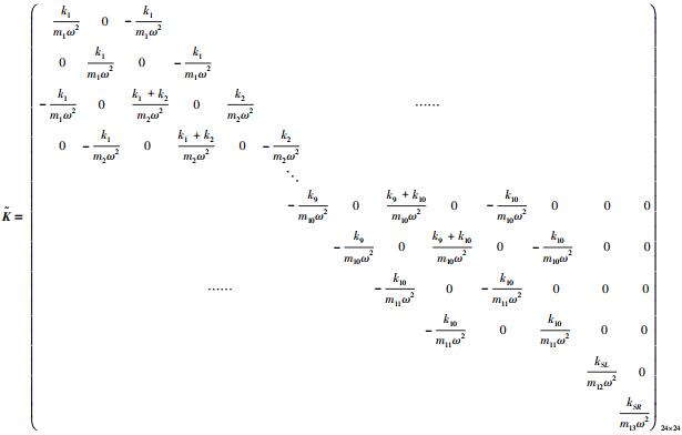
| $ \mathit{\boldsymbol{\tilde K}} = \\{\left( {\begin{array}{*{20}{c}} {{k_1}}&0&{ - {k_1}}&{}&{}&{}&{}&{}&{}&{}&{}&{}&{}&{}&{}\\ 0&{{k_1}}&0&{ - {k_1}}&{}&{}&{}&{}&{}&{}&{}&{}&{}&{}&{}\\ { - {k_1}}&0&{{k_1} + {k_2}}&0&{ - {k_2}}&{}&{}&{}&{}&{}&{ \cdots \cdots }&{}&{}&{}&{}\\ {}&{}&{}&{}&{}& \ddots &{}&{}&{}&{}&{}&{}&{}&{}&{}\\ {}&{}&{}&{}&{}&{}& \ddots &{}&{}&{}&{}&{}&{}&{}&{}\\ {}&{}&{}&{}&{}&{}&{}&{ - {k_9}}&0&{{k_9} + {k_{10}}}&0&{ - {k_{10}}}&0&0&0\\ {}&{}&{}&{}&{}&{}&{}&{}&{ - {k_9}}&0&{{k_9} + {k_{10}}}&0&{ - {k_{10}}}&0&0\\ {}&{}&{}&{}&{ \cdots \cdots }&{}&{}&{}&{}&{ - {k_{10}}}&0&{{k_{10}}}&0&0&0\\ {}&{}&{}&{}&{}&{}&{}&{}&{}&{}&{ - {k_{10}}}&0&{{k_{10}}}&0&0\\ {}&{}&{}&{}&{}&{}&{}&{}&{}&{}&{}&{}&{}&{{k_{SL}}}&0\\ {}&{}&{}&{}&{}&{}&{}&{}&{}&{}&{}&{}&{}&{}&{{k_{SR}}} \end{array}} \right)_{24 \times 24}} $ |
| $ \mathit{\boldsymbol{\tilde F}} = {\left( {\begin{array}{*{20}{c}} {{F_x}\left( {{X_1},{Y_1} - {Y_{12}},{{\dot X}_1},{{\dot Y}_1} - {{\dot Y}_{12}}} \right)}\\ {{F_y}\left( {{X_1},{Y_1} - {Y_{12}},{{\dot X}_1},{{\dot Y}_1} - {{\dot Y}_{12}}} \right) - {m_1}g}\\ {{m_2}{B_2}{\omega ^2}\cos \left( {\omega t} \right)}\\ {{m_2}{B_2}{\omega ^2}\sin \left( {\omega t} \right) - {m_2}g}\\ \vdots \\ {{m_{10}}{B_{10}}{\omega ^2}\cos \left( {\omega t} \right)}\\ {{m_{10}}{B_{10}}{\omega ^2}\sin \left( {\omega t} \right) - {m_{10}}g}\\ {{F_x}\left( {{X_{11}},{Y_{11}},{{\dot X}_{11}},{{\dot Y}_{11}}} \right)}\\ {{F_y}\left( {{X_{11}},{Y_{11}},{{\dot X}_{11}},{{\dot Y}_{11}}} \right) - {m_{11}}g}\\ { - {F_y}\left( {{X_1},{Y_1} - {Y_{12}},{{\dot X}_1},{{\dot Y}_1} - {{\dot Y}_{12}}} \right) - {m_{12}}g}\\ { - {F_y}\left( {{X_1},{Y_1} - {Y_{13}},{{\dot X}_1},{{\dot Y}_1} - {{\dot Y}_{12}}} \right) - {m_{13}}g} \end{array}} \right)_{24 \times 1}},\\ \mathit{\boldsymbol{\bar f}} = {\left( {\begin{array}{*{20}{c}} {\frac{1}{{{M_1}}}{f_x}\left( {{x_1},{y_1} - {y_{12}},{{\dot x}_1},{{\dot y}_1} - {{\dot y}_{12}}} \right)}\\ {\frac{1}{{{M_1}}}{f_y}\left( {{x_1},{y_1} - {y_{12}},{{\dot x}_1},{{\dot y}_1} - {{\dot y}_{12}}} \right) - \frac{g}{{{\omega ^2}c}}}\\ {{b_2}\cos \tau }\\ {{b_2}\sin \tau - \frac{g}{{{\omega ^2}c}}}\\ \vdots \\ {{b_{10}}\cos \tau }\\ {{b_{10}}\sin \tau - \frac{g}{{{\omega ^2}c}}}\\ {\frac{1}{{{M_{11}}}}{f_x}\left( {{x_{11}},{y_{11}},{{\dot x}_{11}},{{\dot y}_{11}}} \right)}\\ {\frac{1}{{{M_{11}}}}{f_y}\left( {{x_{11}},{y_{11}},{{\dot x}_{11}},{{\dot y}_{11}}} \right) - \frac{g}{{{\omega ^2}c}}}\\ { - \frac{1}{{{M_{12}}}}{f_y}\left( {{x_1},{y_1} - {y_{12}},{{\dot x}_1},{{\dot y}_1} - {{\dot y}_{12}}} \right) - \frac{g}{{{\omega ^2}c}}}\\ { - \frac{1}{{{M_{13}}}}{f_y}\left( {{x_1},{y_1} - {y_{13}},{{\dot x}_1},{{\dot y}_1} - {{\dot y}_{13}}} \right) - \frac{g}{{{\omega ^2}c}}} \end{array}} \right)_{24 \times 1}} $ |
|
The dimensionless form can be obtained via nondimensionalizing Eq.(1), and the dimensionless transformation is defined as:
| $ \tau = \omega t,{x_i} = \frac{{{X_i}}}{c},{y_i} = \frac{{{Y_i}}}{c},\dot x = \frac{{{\rm{d}}{x_i}}}{{{\rm{d}}\tau }},\dot y = \frac{{{\rm{d}}{y_i}}}{{{\rm{d}}\tau }},{{\ddot x}_i} = \frac{{{\rm{d}}{{\ddot x}_i}}}{{{\rm{d}}\tau }}, $ |
| $ {{\ddot y}_i} = \frac{{{\rm{d}}{{\dot y}_i}}}{{{\rm{d}}\tau }},{M_1} = \frac{{{m_1}c{\omega ^2}}}{{sP}},{M_{11}} = \frac{{{m_{11}}c{\omega ^2}}}{{sP}},{M_{12}} = \frac{{{m_{12}}c{\omega ^2}}}{{sP}}, $ |
| $ {M_{13}} = \frac{{{m_{13}}c{\omega ^2}}}{{sP}},{b_i} = \frac{{{B_i}}}{c}\left( {i = 2, \cdots ,10} \right),{f_x} = \frac{{{F_x}}}{{sP}},{f_y} = \frac{{{F_y}}}{{sP}} $ |
The parameters above are the same as those in Refs. [24-25, 29].
The dimensionless form of Eq.(1) is expressed as Eq.(2) via the dimensionless transformation, the expression of
| $ \mathit{\boldsymbol{\ddot z}} = - \mathit{\boldsymbol{\bar c\dot z}} - \mathit{\boldsymbol{\bar kz}} + \mathit{\boldsymbol{\bar f}} $ | (2) |
The parameters of the rotor system are expressed in details as follows:
m1=4 kg, m2=21.933 9 kg, m3=7.799 0 kg, m4=6.354 5 kg, m5=9.066 6 kg, m6=5.977 3 kg, m7=5.977 3 kg, m8=6.980 9 kg, m9=7.228 4 kg, m10=3.901 46 kg, m11=4 kg, m12=m13=75 kg, R=L=30 mm, c=0.15 mm, μ=0.018 Pa·s, c1=c11=800 (N·s)/m, c2=c10=1 250 (N·s)/m, c3=c9=1 050 (N·s)/m, c4=c8=850 (N·s)/m, c5=c7=1 050 (N·s)/m, c6=1 650 (N·s)/m, ki=2×10⁷ N/m(i=1, ..., 10, i≠5), kSL1=kSR1=7.5×10⁷ N/m, kSL2=kSR2=2.5×10⁸ N/m, cSL1=cSR1=350 (N·s)/m, cSL2=cSR2=500 (N·s)/m, B5= 0.01 mm, Bi=0(i=2, ...10, i≠5), δ1=δ2=0.22 mm.
Formula (3) shows nonlinear oil-film force[31]of both x and y directions, and detailed parameters are the same as those in Section 3.1 [24].
| $ \begin{array}{l} \left\{ {\begin{array}{*{20}{c}} {{f_x}}\\ {{f_y}} \end{array}} \right\} = \frac{{{{\left[ {\left( {x - 2{{\dot y}^2} + {{\left( {y + 2\dot x} \right)}^2}} \right.} \right]}^{1/2}}}}{{1 - {x^2} - {y^2}}} \times \\ \left\{ \begin{array}{l} 3xV\left( {x,y,a} \right) - \sin \alpha G\left( {x,y,\alpha } \right) - 2\cos \alpha S\left( {x,y,\alpha } \right)\\ 3yV\left( {x,y,a} \right) + \cos \alpha G\left( {x,y,\alpha } \right) - 2\sin \alpha S\left( {x,y,\alpha } \right) \end{array} \right\} \end{array} $ | (3) |
For convenience of theoretical analysis, then the parameter α can be rewritten as formula (4) via Taylor series expansion of the oil-film force:
| $ \begin{array}{l} \alpha = \arctan \frac{{y + 2\dot x}}{{x - 2\dot y}} - \frac{{\rm{ \mathsf{ π} }}}{2}\left( {\frac{{\left. {\left( {y + 2} \right) + 2\dot x} \right)\left( {x - 2\dot y} \right)}}{{\left| {y + 2\dot x} \right|\left| {x - 2\dot y} \right|}}} \right) - \\ \;\;\;\frac{{\rm{ \mathsf{ π} }}}{2}\left( {\frac{{y + 2\dot x}}{{\left| {y + 2\dot x} \right|}}} \right) \end{array} $ | (4) |
Formula (2) is written as Eq. (5) briefly for the convenience of the calculation:
| $ \mathit{\boldsymbol{\ddot Z}} = - \mathit{\boldsymbol{C\dot Z}} - \mathit{\boldsymbol{KZ}} + \mathit{\boldsymbol{F}} $ | (5) |
In Eq.(5), C and K are the damping and stiffness matrixes, F includes oil-film and external excitation etc. Z = (z1, z2, ..., z23, z24) T corresponds to (x1, y1, …, x11, y11, y12, y13)T in Eq.(2).
3 Nonlinear Dynamical Analysis of Rotor System with LoosenessIn this section, the impact of pedestal looseness fault on the rotor-bearing systems is studied. We pay close attention to the vertical direction vibration of the left bearing, and the vertical pedestal looseness has great influence on y1 DOF of the left bearing. The frequency spectrum curves are compared to show the looseness characters. Figs. 4-6 show the time histories of rotor models without looseness, with one end and both ends looseness when the rotating speed is 1 500 rad/s.

|
Figure 4 The y1 DOF time history curve when ω =1 500(rad/s) in the case of without looseness |

|
Figure 5 The y1 DOF time history curve when ω =1 500(rad/s) in the case of with looseness at one end |

|
Figure 6 The y1 DOF time history curve when ω =1 500(rad/s) in the case of with looseness at both ends |
The initial conditions are provided as x2=0.5, y2=0.5, xi=yi=y12=0(i=1, ..., 11, i≠4), the integration step is π/512,

|
Figure 7 Frequency spectrum curves without pedestal looseness |
Fig. 8 represents the frequency spectrum curve of the left bearing with looseness at one end. Compared with Fig. 7 and Fig. 8, looseness fault may cause 4/5X, 3/2X and 5/3X frequency components. In Fig. 8, 2/5X fractional frequency occupies the dominant frequency, so looseness may cause 2/5X harmonic resonance. As is clearly seen in Fig. 8(a) and (b), vertical direction of the left bearing contains more frequency components than the horizontal direction, 3/2X and 5/3X frequency appear in Fig. 8 (b).

|
Figure 8 Frequency spectrum curves of left end looseness model |
The frequency spectrum curves in Fig. 9 are similar as the rotor system model with one end looseness (Fig. 8). The x1 and y1 DOF vibrations are highlighted, the bearing looseness at right end affects little to the left end, so the dynamics behaviors do not vary significantly in comparison to frequency components in Fig. 8.

|
Figure 9 Frequency spectrum curves both ends looseness model |
Remark 1 The units of frequency and amplitude are radian per second, millimeter respectively in this paper, and the rotating speed is chosen as 1 500 rad/s. The oil-film force will generate to 2/5X and 3/5X frequency components, see details in Fig. 7. The pedestal looseness is considered in the direction of gravity, so there is larger effect on the y1 DOF, the 3/2X and 5/3X fractional frequencies occur in Fig. 8(b) and 9(b). The looseness will also lead to 2/5X harmonic resonance via comparing the looseness-free model (Fig. 7) with the fault models (Fig. 8 and Fig. 9).
4 Effect of Initial Values to Frequency ComponentThe effect of initial values on frequency component of three rotor-bearing systems will be studied. Two initial value cases of are chosen to discuss the impact of initial values:one is displacement, the other is velocity. We will choose two sets of initial values based on each case.
4.1 The Case of Displacement VariationFirst, we will study the case of the variation of displacement. Compared with the initial conditions in Section 3, we will change the displacements as x2=y2=0.2 and x2=y2=0.4, the other values are invariant. Figs. 10-12 are frequency-spectrum curves of x1 and y1 DOF of three rotor-bearing systems.

|
Figure 10 Frequency spectrum curves of 22-DOFs rotor system |

|
Figure 11 Frequency spectrum curves of 23-DOFs rotor system |

|
Figure 12 Frequency spectrum curves of 24-DOFs rotor system |
There is only X frequency component in Fig. 10 when we turn the initial values of displacement to 0.2 and 0.4 respectively via comparing with Fig. 7. Initial values have great effect on 22-DOF rotor system without looseness.
In Fig. 11, the frequency components are the same as those in Fig. 8. Initial displacement values have little effect on 23-DOF system with one end looseness. In Fig. 12, there is a great effect to the frequency component when we choose the initial values as 0.2, for the case of initial values 0.4, there is no effect, all the components left compared with Fig. 9.
4.2 The Case of Velocity VariationSecond, the case of the variation of velocity will be studied. Compared with the initial conditions in Section 3, we will change the velocity as

|
Figure 13 Frequency spectrum curves of 22-DOFs rotor system |

|
Figure 14 Frequency spectrum curves of 23-DOFs rotor system |

|
Figure 15 Frequency spectrum curves of 24-DOFs rotor system |
In Fig. 13, when the initial values are chosen as 0.002, the frequency components keep the same as that in Fig. 7. If the velocity has a larger variation (the initial values of velocity is 0.005), there is only X frequency component left in Fig. 13 (c) and Fig. 13 (d).
The frequency spectrum curves of 23 and 24-DOFs systems with different initial values (0.02 and 0.05) of velocity respectively, shown in Figs. 14 and 15, indicate that the frequency components keep the same as Figs. 8 and 9.
To sum up Section 4.1 and 4.2, initial values of displacements have a greater effect than velocities. But larger variation of initial values will have a greater effect to the frequency components. For example, in Fig. 12, the displacements (0.5) are changed as 0.4 and 0.2 respectively, Fig. 12 (a), (b) lose the frequency components and Fig. 12 (c), (d) keep the components relative to the original frequency spectrum curve (Fig. 9). The effect of velocity can be seen clearly in Fig. 13.
Remark 2 The variation of the displacement affects more to dynamical models than the velocity variation, see the 22DOF model in details, the fractional frequencies disappear. If the initial values have a fast-varying (displacement changes from 0.5 to 0.2, velocity from 0.01 to 0.05), the frequency components will change at the same time.
5 Efficiency of TPOD MethodThe dynamics behaviors of the original and the reduced systems are highlighted in this section. The efficiency of the TPOD method is verified via the comparisons of amplitude frequency and bifurcation behaviors. The basic process of the TPOD method is introduced in the authors' previous work, see details in Refs. [24-25, 29-30].
The motion equation of the simplified model can be obtained as the steps above. A 6-DOFs reduced model is obtained by the dimension reduction method, the 6-DOFs reduced system can be written as Eq.(6):
| $ \mathit{\boldsymbol{\ddot P}} = - {\mathit{\boldsymbol{C}}_6}\mathit{\boldsymbol{\dot P}} - {\mathit{\boldsymbol{K}}_6}\mathit{\boldsymbol{P}} + {\mathit{\boldsymbol{F}}_6} $ | (6) |
The damping, stiffness, external excitation matrix are C6, K6, F6, the coefficients of the matrixes are expressed as follows:
| $ {\mathit{\boldsymbol{C}}_6} = \left( {\begin{array}{*{20}{c}} {{c_{11}}}&{{c_{12}}}&{{c_{13}}}&{{c_{14}}}&{{c_{15}}}&{{c_{16}}}\\ {}&{{c_{22}}}&{}&{}&{}&{}\\ {}&{}&{{c_{33}}}&{}&{}&{}\\ {}&{}&{}&{{c_{44}}}&{}&{}\\ {}&{}&{}&{}&{{c_{55}}}&{}\\ {}&{}&{}&{}&{}&{{c_{66}}} \end{array}} \right) $ |
| $ {\mathit{\boldsymbol{K}}_6} = \left( {\begin{array}{*{20}{c}} {{k_{11}}}&{{k_{12}}}&{{k_{13}}}&{{k_{14}}}&{{k_{15}}}&{{k_{16}}}\\ {}&{{k_{22}}}&{}&{}&{}&{}\\ {}&{}&{{k_{33}}}&{}&{}&{}\\ {}&{}&{}&{{k_{44}}}&{}&{}\\ {}&{}&{}&{}&{{k_{55}}}&{}\\ {}&{}&{}&{}&{}&{{k_{66}}} \end{array}} \right) $ |
| $ {\mathit{\boldsymbol{F}}_6} = \left( {\begin{array}{*{20}{c}} {{f_1} + {f_{\omega 1}} + {g_1}}\\ {{f_2} + {f_{\omega 2}} + {g_2}}\\ {{f_3} + {f_{\omega 3}} + {g_3}}\\ {{f_4} + {f_{\omega 4}} + {g_4}}\\ {{f_5} + {f_{\omega 5}} + {g_5}}\\ {{f_6} + {f_{\omega 6}} + {g_6}} \end{array}} \right) $ |
The amplitude-frequency curves and bifurcation diagrams are analyzed to show the efficiency of the TPOD method. The reduced system can preserve the dynamical topological structures of the original one via comparing the original system with the reduced system.
Figs. 16(a)-18(a) show the amplitude frequency curves of the original systems in three situations without pedestal looseness, with one end looseness and with that at both ends respectively. Figs. 16(b)-18(b) show the amplitude-frequency curves of the reduced systems obtained by TPOD method. Figs. 16(b)-18(b) demonstrate that the reduced systems reserve the main amplitude frequency behaviors of original systems, especially the 24-DOF rotor model.

|
Figure 16 Amplitude-frequency curves without pedestal looseness |

|
Figure 17 Amplitude-frequency curves with one end pedestal looseness |

|
Figure 18 Amplitude-frequency curves with both ends pedestal looseness |
Figs. 19-21 provide the bifurcation diagrams of the original and the simplified systems. Figs. 19(a)-21(a) show the bifurcation behaviors of the original systems and Figs. 19(b)-21(b) show those of the reduced system obtained by the order reduction method. Figs. 19(b)-21(b) show that the reduced systems maintain the main dynamical behaviors of the original ones. Again, in Fig. 19(b), though the reduced system reserves the main dynamics behaviors, it also loses some dynamical characters, there is a delay interval compared with the original bifurcation diagram (Fig. 19(a)).

|
Figure 19 Bifurcation diagrams without pedestal looseness |

|
Figure 20 Bifurcation diagrams with left end pedestal looseness |

|
Figure 21 Bifurcation diagrams with both ends pedestal looseness |
In Fig. 20, the rotor model with pedestal looseness causes more complex bifurcation behavior than the model without looseness. In Fig. 21, the motion behavior of the system with both ends pedestal looseness is more complex than one end looseness. Fig. 21(b) also indicates that the diagram keeps basically the same as the original system in the whole interval. The results show that the transient POD method is more suitable in the more complex rotor system.
Based on the study of original initial values, the effect of variation of initial values to the efficiency of the dimension reduction method will be discussed here.Figs. 22-24 show the y1 DOF bifurcation diagrams of three different reduced rotor systems respectively. In Fig. 22, it shows the bifurcation diagrams with different initial values. Figs. 22(a), (b), (c), (d) are the cases with initial values of displacement 0.2, 0.4 and velocity 0.02, 0.05 respectively. Figs. 23, 24 are similar as Fig. 22.

|
Figure 22 Bifurcation diagrams without pedestal looseness |

|
Figure 23 Bifurcation diagrams with left end pedestal looseness |

|
Figure 24 Bifurcation diagrams with both ends pedestal looseness |
As is clearly indicated in Fig. 22, the four bifurcation diagrams with different initial values cannot maintain similar structure of the original rotor system (Fig. 19 (a)). So the reduced systems cannot maintain dynamics behaviors of the original one. The initial values variations have the effect to order reduction efficiency.
Figs. 23 and 24 are the bifurcation diagrams with different initial values of 23-DOFs and 24-DOFs systems. The bifurcation behaviors indicate that the reduced systems can not reserve main dynamics behaviors of the original ones.
The dimension reduction efficiency of TPOD method is verified through the comparisons between the amplitude-frequency curves, bifurcation characteristics of both the original and simplified models. The results show that the initial conditions have great effects to order reduction efficiency. This dimension reduction method is more suitable in strongly nonlinear systems.
Remark 3 On the basis of three rotor models, the efficiency of the TPOD method is verified via comparing the amplitude-frequency curves and the bifurcations of the original and reduced models. The order reduction method is more suitable in the complex rotor model (24-DOF model). The initial values variations have a large effect to the bifurcation behaviors. The topological structures of bifurcation of the original models cannot be reserved.
6 ConclusionsThe dynamic behaviors of pedestal looseness fault of the reduced rotor-bearing system have been analyzed in this paper. We have established rotor-bearing models without pedestal looseness, with looseness at one end and that at both ends respectively. Pedestal looseness may cause fractional frequency vibration, such as 4/5X, 3/2X, 5/3X and 2/5 harmonic vibration. The nonlinear TPOD method has been used to reduce the multi-DOFs models to the 6-DOFs ones which reserve the dynamical behaviors of the original ones via comparing with amplitude-frequency curves and bifurcation diagrams. The initial value variation affects little to the order reduction efficiency based on the qualitative aspect, but a larger effect to the frequency components. The reduced models provide convenience for the qualitative analysis of the original ones. Further works will be presented as follows: one is to use the experiment to verify the numerical results; then the dimension reduction method will be generated to the dual-rotor system; finally, the uncertainties in the rotor system will be highlighted.
AcknowledgementsThe authors would like to acknowledge the support of the China Scholarship Council and the guidance of professor Sharif Rahman in the University of Iowa.
| [1] |
Chu F L, Tang Y. Stability and nonlinear responses of a rotor-bearing system with pedestal looseness. Journal of Sound and Vibration, 2001, 241(5): 879-893. DOI:10.1006/jsvi.2000.3341 (  0) 0) |
| [2] |
Ma H, Zhao X Y, Teng Y N, et al. Analysis of dynamic characteristics for a rotor system with pedestal looseness. Shock and Vibration, 2011, 18(1-2): 13-27. DOI:10.1155/2011/753047 ( 0) |
| [3] |
Ji Z, Zu J W. Method of multiple scales for vibration analysis of rotor-shaft systems with non-linear bearing pedestal model. Journal of Sound and Vibration, 1998, 218(2): 293-305. DOI:10.1006/jsvi.1998.1835 ( 0) |
| [4] |
Hou L, Chen Y S, Cao Q J. Nonlinear vibration phenomenon of an aircraft rub-impact rotor system due to hovering flight. Communications in Nonlinear Science and Numerical Simulation, 2014, 19(1): 286-297. DOI:10.1016/j.cnsns.2013.06.023 ( 0) |
| [5] |
Chu F L, Liu W X. Experimental observation of nonlinear vibrations in a rub-impact rotor system. Journal of Sound and Vibration, 2005, 283(3-5): 621-643. DOI:10.1016/j.jsv.2004.05.012 ( 0) |
| [6] |
Chu F L, Zhang Z. Bifurcation and chaos in a rub-impact Jeffcott rotor system. Journal of Sound and Vibration, 1998, 210(1): 1-18. DOI:10.1006/jsvi.1997.1283 ( 0) |
| [7] |
Lu Q S, Li Q H, Twizell E H. The existence of periodic motions in rub-impact rotor systems. Journal of Sound and Vibration, 2003, 264(5): 1127-1137. DOI:10.1016/S0022-460X(02)01386-X ( 0) |
| [8] |
Chu F L, Zhang Z S. Periodic, quasi-periodic and chaotic vibrations of a rub-impact rotor system supported on oil film bearings. International Journal of Engineering Science, 1997, 35(10-11): 963-973. DOI:10.1016/S0020-7225(97)89393-7 ( 0) |
| [9] |
Hou L, Chen Y S, Lu Z Y, et al. Bifurcation analysis for 2:1 and 3:1 super-harmonic resonances of an aircraft cracked rotor system due to maneuver load. Nonlinear Dynamics, 2015, 81(1-2): 531-547. DOI:10.1007/s11071-015-2009-1 ( 0) |
| [10] |
AL-Shudeifat M A, Butcher E A, Stern C R. General harmonic balance solution of a cracked rotor-bearing-disk system for harmonic and sub-harmonic analysis: Analytical and experimental approach. International Journal of Engineering Science, 2010, 48(10): 921-935. DOI:10.1016/j.ijengsci.2010.05.012 ( 0) |
| [11] |
AL-Shudeifat M A, Butcher E A. New breathing functions for the transverse breathing crack of the cracked rotor system: Approach for critical and subcritical harmonic analysis. Journal of Sound and Vibration, 2011, 330(3): 526-554. DOI:10.1016/j.jsv.2010.08.022 ( 0) |
| [12] |
Han Q K, Chu F L. Parametric instability of a Jeffcott rotor with rotationally asymmetric inertia and transverse crack. Nonlinear Dynamics, 2013, 73(1-2): 827-842. DOI:10.1007/s11071-013-0835-6 ( 0) |
| [13] |
Li B, Chow M Y, Tipsuwan Y, et al. Neural-network-based motor rolling bearing fault diagnosis. IEEE Transactions on Industrial Electronics, 2000, 47(5): 1060-1069. DOI:10.1109/41.873214 ( 0) |
| [14] |
Rai V K, Mohanty A R. Bearing fault diagnosis using FFT of intrinsic mode functions in Hilbert-Huang transform. Mechanical Systems and Signal Processing, 2007, 21(6): 2607-2615. DOI:10.1016/j.ymssp.2006.12.004 ( 0) |
| [15] |
Prabhakar S, Mohanty A R, Sekhar A S. Application of discrete wavelet transform for detection of ball bearing race faults. Tribology International, 2002, 35(12): 793-800. DOI:10.1016/S0301-679X(02)00063-4 ( 0) |
| [16] |
Lees A W. Misalignment in rigidly coupled rotors. Journal of Sound and Vibration, 2007, 305(1-2): 261-271. DOI:10.1016/j.jsv.2007.04.008 ( 0) |
| [17] |
AL-Hussain K M, Redmond I. Dynamic response of two rotors connected by rigid mechanical coupling with parallel misalignment. Journal of Sound and Vibration, 2002, 249(3): 483-498. DOI:10.1006/jsvi.2001.3866 ( 0) |
| [18] |
Muszynska A, Goldman P. Chaotic responses of unbalanced rotor/bearing/stator systems with looseness or rubs. Chaos, Solitons & Fractals, 1995, 5(9): 1683-1704. DOI:10.1016/0960-0779(94)00171-L ( 0) |
| [19] |
Goldman P, Muszynska A. Analytical and experimental simulation of loose pedestal dynamic effects on a rotating machine vibrational response. Rotating Machinery Dynamics, DE-Vol. 35, The 13th Biennial ASME Conference on Mechanical Vibration and Noise. Florida, 1991, 35: 11-17. ( 0) |
| [20] |
Rega G, Troger H. Dimension reduction of dynamical systems:methods, models, applications. Nonlinear Dynamics, 2005, 41(1-3): 1-15. DOI:10.1007/s11071-005-2790-3 ( 0) |
| [21] |
Steindl A, Troger H. Methods for dimension reduction and their application in nonlinear dynamics. International Journal of Solids and Structures, 2001, 38(10-13): 2131-2147. DOI:10.1016/S0020-7683(00)00157-8 ( 0) |
| [22] |
Liang Y C, Lee H P, Lim S P, et al. Proper orthogonal decomposition and its applications, part Ⅰ: Theory. Journal of Sound and Vibration, 2002, 252(3): 527-544. DOI:10.1006/jsvi.2001.4041 ( 0) |
| [23] |
Yu H, Chen Y S, Cao Q J. Bifurcation analysis for nonlinear multi-degree-of-freedom rotor system with liquid-film lubricated bearings. Applied Mathematics and Mechanics, 2013, 34(6): 777-790. DOI:10.1007/s10483-013-1706-9 ( 0) |
| [24] |
Lu K, Yu H, Chen Y S, et al. A modified nonlinear POD method for order reduction based on transient time series. Nonlinear Dynamics, 2015, 79(2): 1195-1206. DOI:10.1007/s11071-014-1736-z ( 0) |
| [25] |
Lu K, Jin Y L, Chen Y S, et al. Stability analysis of reduced rotor pedestal looseness fault model. Nonlinear Dynamics, 2015, 82(4): 1611-1622. DOI:10.1007/s11071-015-2264-1 ( 0) |
| [26] |
Kerschen G, Golinval J C, Vakakis A F, et al. The method of proper orthogonal decomposition for dynamical characterization and order reduction of mechanical systems: An overview. Nonlinear Dynamics, 2005, 41(1-3): 147-169. DOI:10.1007/s11071-005-2803-2 ( 0) |
| [27] |
Smith T R, Moehlis J, Holmes P. Low-dimensional modeling of turbulence using the proper orthogonal decomposition: A tutorial. Nonlinear Dynamics, 2005, 41(1-3): 275-307. DOI:10.1007/s11071-005-2823-y ( 0) |
| [28] |
Kerschen G, Golinval J C. Physical interpretation of the proper orthogonal modes using the singular value decomposition. Journal of Sound and Vibration, 2002, 249(5): 849-865. DOI:10.1006/jsvi.2001.3930 ( 0) |
| [29] |
Lu K, Chen Y S, Jin Y L, et al. Application of the transient proper orthogonal decomposition method for order reduction of rotor systems with faults. Nonlinear Dynamics, 2016, 86(3): 1913-1926. DOI:10.1007/s11071-016-3004-x ( 0) |
| [30] |
Lu K, Chen Y S, Cao Q J, et al. Bifurcation analysis of reduced rotor model based on nonlinear transient POD method. International Journal of Non-Linear Mechanics, 2016, 89: 83-92. DOI:10.1016/j.ijnonlinmec.2016.11.013 ( 0) |
| [31] |
Adiletta G, Guido A R, Rossi C. Chaotic motions of a rigid rotor in short journal bearings. Nonlinear Dynamics, 1996, 10(3): 251-269. DOI:10.1007/BF00045106 ( 0) |