In the mobile robot mapping, a robot uses sensors to collect data and further to build up its environment map. To build a map, the robot requires a good estimation of localization and the external environment information got on its pose. While for localization, the robot needs a known map. Therefore, these two problems are described as a "chicken-and-egg" problem. Regarding the problem of localization with a known map, a solution has been proposed in Ref.[1]. In contrast, in simultaneous localization and mapping (SLAM)[2], a mobile robot starts from an unknown initial configuration (position and posture) in an unknown environment. The robot uses sensed information to construct utilizing incremental map while conducts self-position location. The basic idea is that the mobile robot creates a map using a series of its positions, and in turn takes advantage of the map in creating to locate itself. In other words, mapping and localization are simultaneous.
The earliest method to solve the SLAM problem is based on extended Kalman filter (EKF)[3], it estimates the robot pose and mapping in a high-dimensional state space, in order to estimate the possible states of the robot. Li et al.[4] analyzed the EKF consistency issues, and had noted the inconsistent phenomenon with the EKF algorithm due to the linearization error. Also, Doucet[5] proposed a method based on RBPF to solve SLAM effectively by separating a SLAM problem into an estimation of n-paths and independent landmark associated with the assumed path.
Particle Filter (PF) are also applied to solve and improve the efficiency of SLAM. Grisetti et al.[6] presented a grid map representation algorithm and proposed the FastSLAM. Further, FastSLAM algorithm was successfully applied to feature map[7]. Li et al.[8] proposed an algorithm of multi-particle jointly maintaining a map, overcoming the original idea that updating and maintaining the map of each particle individually. As for improving the efficiency and accuracy, Pei et al.[9] proposed a method based on distributed structure to overcome the drawbacks of FastSLAM. Song[10] et al. presented the CFastSLAM and the improved SRCFastSLAM[11]. In recent years, many research focused on vision-SLAM[12-13], VI-SLAM and 3D-SLAM[14] are presented, most of them are graph-based SLAM algorithm and suffering the lack of robust compared with the multi-hypothesis of PF-based algorithm.
In recent years, many researches focused on optimization SLAM[12-14] are presented, most of them are Visual SLAM algorithms instead of LiDAR SLAM algorithms. For the LiDAR based SLAM, whose sensor feedback has no texture information compared with vision, it is harder to build up the data association correctly and localize globally without the multi-hypothesis of PF algorithm.
Although many researches have been done on FastSLAM, little work has been conducted on the data structure of particles. As an important method for global localization, the study of RBPF is very valuable. Inspired by the Ref.[8], in order to solve the problem that particles have a large computational consumption because of individual mapping, a non-intact particle data algorithm is proposed in this paper. The simulation and experiment have verified the accuracy and efficiency of the presented algorithm. In the meanwhile, it saves the size of occupied data compared with the original FastSLAM algorithm.
In this work, we propose an improved algorithm based on original FastSLAM algorithm after analysis its flaws in Section 2-3, and we apply this improved algorithm to simulation and experiment in Section 4 and Section 5. The conclusions are stated in Section 6.
2 FastSLAM 2.1 Introduction to FastSLAMIn FastSLAM, estimation of the robot pose and the map are mutually dependent and alternately calculated, different from the Kalman Filter (KF) algorithm. For the convenience of expression and consistency with common expression, the text representation of all data here is the same as that in Ref.[15], where x is the robot's status, m is the map, z is the observation from LiDAR and u is the control. In addition, the subscript of symbols is the correspondent timestamp. Consequently, SLAM problem can be expressed as the problem of solving the estimation of the probability
| $ \begin{array}{l} p\left( {{x_{1:t}},m\left| {{z_{1:t}}} \right.,{u_{0:\left( {t - 1} \right)}}} \right) = p\left( {{x_{1:t}}\left| {{z_{1:t}}} \right.,{u_{0:\left( {t - 1} \right)}}} \right) \cdot \\ \;\;\;\;\;\;\;\;\;p\left( {m\left| {{x_{1:t}}} \right.,{z_{1:t}}} \right) \end{array} $ | (1) |
where
By the formula (1), we can calculate the localization estimation
The main steps of FastSLAM are listed as follows:
(A) Sampling the particles set from the proposal distribution.
(B) Computing the importance weights: using observation model to assign each particle a weight.
(C) Resampling: taking the effective number of particles Neff as a criterion whether resampling. According to the weights of particles, larger weights particles replace the smaller ones. After resample, all particles have equal weights.
(D) Map updating: according to the known position and observation, the map information of each particle is updated.
2.2 Shortcomings of FastSLAM AlgorithmAs mentioned above, an individual map is saved within each particle in FastSLAM, which takes a great deal of memory space and computational consumption. These shortcomings are more serious when the FastSLAM algorithm is applied to the grid map in Ref.[6]. Using a grid map representation, each particle carries a great amount of data. In order to control the amount of data, the size of the particle set must be strictly controlled. Much related work has been presented to control the size of the particle set and improve the quality of the SLAM, including improving the distribution of the proposed algorithm[12], using the effective number of particles to resample selectively[6] and so on.
As a general characteristic of Particle Filter, if and only if the size of particle set tends to be infinite, the estimated distribution approximates the real one. As can be seen from the convergence condition, the contradiction between computation and the size of the particle set presents in the practical application for FastSLAM algorithm. On the one hand, each particle carries a large amount of data about the map information, which requires a lot of computation and exhausts large memory space. It is necessary to control the particle size strictly. On the other hand, due to the characteristics of PF, only when the number of particles tends to be infinity, does the estimated distribution approach to the true distribution. It is a serious confliction.
Some methods are proposed to improve the efficiency of particle based SLAM algorithm, including utilizing a strategy of multi-robots[18-19] and considering odometer information for particles updating[20]. However, little work focuses on the confliction mentioned above. A non-intact particle data algorithm is proposed to resolve this confliction.
3 Non-Intact Particle Data RBPFSince the non-particle data algorithm is studied based on the FastSLAM, this section introduces MCL algorithm and mapping algorithms applied to FastSLAM algorithm firstly. Non-intact particle data RBPF based on them is then proposed.
3.1 Monte Carlo Localization AlgorithmMCL is applied to the FastSLAM algorithm to estimate
| $ B\left( {{x_t}} \right) = \eta \cdot p\left( {{z_t}\left| {{x_t}} \right.} \right) \cdot \int {p\left( {{x_t}\left| {{u_t}} \right.,{x_{t - 1}}} \right)B\left( {{x_{t - 1}}} \right){\rm{d}}{x_{t - 1}}} $ | (2) |
As Eq.(2) shows, B(x1) is the believability that obtained from B(xt-1) by iteration. The kinematic model
Because of RBPF separation, the problem of mapping under the unknown pose is transformed into the mapping based on the known pose. Such algorithms have been proposed in previous studies[15-17], with either grid map or landmark map. They all apply Bayesian iteration to update the map. Since the algorithm that proposed in this paper does not care about its detail, the detail of mapping algorithm is not introduced here.
To facilitate analysis of the error and statistics, the landmark map is applied. And the expressions of formulas below also take landmark map representation as the analysis objects. The landmark map information (prediction and update matrixes) that particles saves is defined as follows:
| $ \left\{ \begin{array}{l} {\mathit{\boldsymbol{p}}_f},{\rm{prediction}}\;{\rm{landmark}}\;{\rm{matrix}}\\ {\mathit{\boldsymbol{x}}_f},{\rm{updated}}\;{\rm{landmark}}\;{\rm{matrix}} \end{array} \right. $ | (3) |
Compared with the original algorithm, the main differences between the non-intact particles data algorithm and the original algorithm is that after the completion of robot position and posture estimation, the former does not directly estimate the map. A filter is taken for the particles that carry pose information and the larger weights to obtain a particle set. Only those particles carrying individual maps are updated. In this algorithm, the particles that carry the complete information (including individual map and pose information) are called the primary particles.
The filter of the primary particles and its associated processes are described in detail below. Firstly, the first iteration of the non-intact particle data algorithm is the same as the original one. All of the particles are involved in the localization, weight calculation and mapping operations. After the first iteration, the particle selection is performed to obtain particles with a large weight by filter function. This set is called the primary particle set, denoted as Xeff. And in the subsequent steps, only the primary particle set is involved in mapping and map updating processes to reduce the consumption caused by mapping process and its update. Meanwhile, the initial set of particles is retained in order to complete the iteration step. While coding and programing, no additional memory space is needed for Xeff, only by adding a mark into the original particles to reduce the occupied memory.
The filter function is described in detail below. The number of effective particles Neff in resampling process is represented as a size parameter of the primary particle sets, where
| $ {N_{{\rm{eff}}}} = \frac{1}{{\sum\limits_{i = 1}^N {{{\left( {{W^i}} \right)}^2}} }} $ | (4) |
The size of the primary particle set can be expressed as Neff·d-1, where d is applied to control the size of Xeff. Meanwhile, a function
| $ {\mathit{\boldsymbol{X}}_{{\rm{eff}}}} = \mathop {\max }\limits_{{N_{{\rm{eff}}}} \cdot {d^{ - 1}}} \left( \mathit{\boldsymbol{X}} \right) $ | (5) |
As can be seen, d controls the diversity of the individual exactly, which determines the size of data and the accuracy of map to a certain extent. In addition, as formula (5) shows, this step must be completed prior to resampling. Because each particle carries an average weight after resample, which cannot be filtered to get the primary particles according to their weights.
3.3.2 Data complement of the secondary particle setAs described in the previous sections, in the non-intact particles data algorithm, the data structure that each particle carries may be different. Only the primary particle set carries the complete information. The particles with small weights carry the position and posture information only, but no individual map, such particles set is called the secondary particles in this paper. By RBPF algorithm and iteration of Bayesian algorithm, as shown in the formula (2), the next generation of particles is obtained from the posterior generation. In order to run the iteration successfully, the data structure of the secondary particle set must be completed by a "pseudo-complete data structure" in order to involve in the algorithm iteration of the original algorithm. Here, this step is called "data complement of the secondary particle set".
The basic idea of data complement is that copying the individual maps that the primary particle set carries, and spreading them in the secondary particle set, that is, covering the two matrices pf and xf in Eq.(3). The initial particles set, the primary particle set and the secondary particle set is denoted as X, Xeff and Xuneff respectively, then
| $ \mathit{\boldsymbol{X}} = {\mathit{\boldsymbol{X}}_{{\rm{uneff}}}} \cup {\mathit{\boldsymbol{X}}_{{\rm{eff}}}} $ | (6) |
The individual particles in Xeff and Xuneff are denoted as Xeffi and Xuneffj, then the data complement steps can be expressed as follows:
| $ \begin{array}{l} \mathit{\boldsymbol{X}}_{{\rm{uneff}}}^i \cdot {\mathit{\boldsymbol{p}}_f} = X_{{\rm{eff}}}^{\left( {ceil\left( {{\alpha ^i}/\beta } \right)} \right)} \cdot {\mathit{\boldsymbol{p}}_f}\\ \mathit{\boldsymbol{X}}_{{\rm{uneff}}}^i \cdot {\mathit{\boldsymbol{x}}_f} = X_{{\rm{eff}}}^{\left( {ceil\left( {{\alpha ^i}/\beta } \right)} \right)} \cdot {\mathit{\boldsymbol{x}}_f} \end{array} $ | (7) |
where ceil(x)=[x]+1
| $ \begin{array}{*{20}{c}} {\beta = \left( {size\left( \mathit{\boldsymbol{X}} \right) - size\left( {{\mathit{\boldsymbol{X}}_{{\rm{eff}}}}} \right) \cdot {d^{ - 1}}} \right) \cdot \left( {size\left( {{\mathit{\boldsymbol{X}}_{{\rm{eff}}}}} \right) \cdot } \right.}\\ {{{\left. {{d^{ - 1}}} \right)}^{ - 1}} = \frac{{size\left( \mathit{\boldsymbol{X}} \right) \cdot diff}}{{size\left( {{\mathit{\boldsymbol{X}}_{{\rm{eff}}}}} \right)}} - 1} \end{array} $ | (8) |
| $ {\alpha ^i} = i - size\left( {{\mathit{\boldsymbol{X}}_{{\rm{eff}}}}} \right) \cdot {d^{ - 1}} $ | (9) |
The function ceil(x) makes the results in formula (8) and (9) an integer one, which can be regarded as an index of particles to involve in the formula (7). After the steps above, the map information of Xeff is spread to Xuneff evenly, all the particles have got a pseudo complete data, which can be substituted into Eqs.(1) and (2) to achieve the iteration of RBPF algorithm formulas.
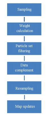
3.3.3 Pipeline and the complexityThe non-intact particle data algorithm is achieved by the idea mentioned above, the pipeline is shown in Fig. 1.
|
Figure 1 Steps of non-intact particle data algorithm |
(A) Sampling: according to the proposed distribution, the samples are obtained randomly.
(B) Weight calculation: assigning each particle an important weight.
(C) Get the primary and secondary particle set by filter, obtaining the primary particles and secondary particle sets according to formulas (5) and (6).
(D) Data complement of the secondary particle set, each of the secondary particle data is completed for the subsequent iterations according to formula (7).
(E) Resampling: according to the weights and using Neff as a criterion to determine whether or not to run the resampling process, the particles with larger weights take place the particles with lower weights, and the average of the weights is taken as the new weight after resample.
(F) Map updates: only the primary particle set obtained in step (C), the individual maps are updated.
As for the analysis of computational complexity, the Particle Filter operation is actually a sort function, whose complexity is O(n·log2n), and the complexity of data complement process is O(n). In addition, due to the computational complexity of mapping decreased from O(n·log2(M)) to O(Neff·log2n), where M is the size of the map, compared with the original method, the new algorithm reduces the computational burden considerably.
4 Simulations 4.1 Simulation ResultsSimulations are based on LiDAR-based FastSLAM 2.0, and the algorithm is implemented with Matlab on a computer with a 3.2 GHz Intel quad-core CPU and 4 GB memory. Random errors are introduced into control and sensor observation.
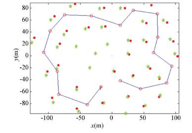
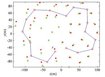
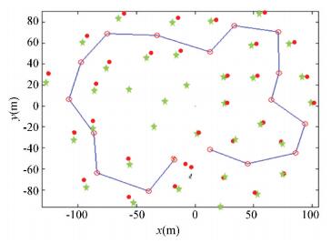
The simulation results and the corresponding landmarks error are shown in Fig. 2-Fig. 6, where the stars are the given landmarks, the line is the movement path and the points are the estimated landmarks in the algorithm, the unit of the map size is meter. The map is built with 35 landmarks, which are distributed around the movement path. And the movement path is given by 17 positions (the circles). The error shown in Fig. 6, it is the sum of Euclidean distance between each true landmarks pm(xy)T and estimated landmarks xf(xy)T. For particle k, the mapping error ekm is calculated by the followed formula,
| $ e_k^m = \sum\limits_{i = 1}^N {{{\left\| {{\mathit{\boldsymbol{x}}_\mathit{\boldsymbol{f}}} - {\mathit{\boldsymbol{p}}_\mathit{\boldsymbol{m}}}} \right\|}^2}} $ | (10) |
|
Figure 2 With the original FastSLAM, n=100 |
|
Figure 3 With the new FastSLAM, n=100 |
|
Figure 4 With the new FastSLAM, n=150 |
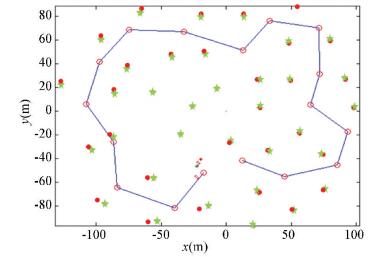
|
Figure 5 With the new FastSLAM, n=200 |
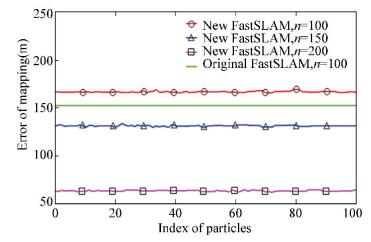
|
Figure 6 Mapping error |
where N is the number of landmarks.
To analyze the computation rate, we carry out time consume analysis by using a set of particles size. At the same time, we define the quantitative value d by using the linear function as:
| $ d = \left( {n - {n_0}} \right) \cdot \alpha + \beta $ | (11) |
where α=0.002, β=2, n0=100. By linear fitting of discrete points, the computation time consume is obtained and shown in Fig. 7.
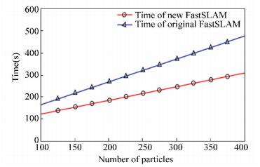
|
Figure 7 Comparison of time consumption |
4.2 Analysis of the Simulation
In terms of mapping accuracy, as shown in Figs. 2-6, under the condition of the same particles size, this algorithm has error increment of 16% than the original FastSLAM algorithm. In addition, similar to the original algorithm, the accuracy of mapping is improved with the increment of particles size. With regard to time consumption, as shown in Fig. 7, under the same number of particles, this algorithm is superior in speed, and the speed advantage became more significant with the increment of particle collection. Compared with the original algorithm, the computing time is decreased by 18%-34% under the same size of particle.
From the simulation results, we can draw the conclusion:
(A) Under the condition of the same computing time, we can use more particles than the original algorithm in order to improve the accuracy of mapping;
(B) Under the condition of the same particles size, the computing efficiency is increased at the expense of reducing composition accuracy to some extent;
(C) The graph of particle variance in the new algorithm has more significant jitter than the original one.
Regarding memory space occupation, it cannot be directly analyzed in the simulation, but since the secondary particle set does not carry individual map information, it only clones the map information carried by the primary ones. Therefore, it is easy to know that the individual map data turns to
The "Victoria Park" dataset is used as the experimental dataset here, which is a classical landmarks-based LiDAR dataset, as shown in Fig. 8. For verifying the non-intact RBPF algorithm, a comparative experiment is established. We set original RBPF with 100 particles, non-intact RBPF with 100 particles and 200 particles to perform the comparison.
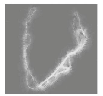
|
Figure 8 The experiment result |
Compared with the simulation mentioned above, whose number of landmarks is 35, the number of landmarks in Victoria Park dataset is much more. It is almost impossible to calculate the mapping error according to the data association of landmarks and observation, result from the outlier of data association. Therefore, the analysis of error is calculated by the sum of localization error within some sampled positions instead of all the pose points. However, the localization error and the mapping error have a similar meaning in landmarks-based SLAM to some extent.
In this experiment, nine positions are selected randomly to measure the accuracy of the algorithm, which distribute along the whole moving path. The localization error el is calculated by the followed formula, where W is the number of selected way points, pe(xy)T is the estimated position of the highest weight particle, and wp(xy)T is the way point.
| $ {e^l} = \sum\limits_{i = 1}^W {{{\left\| {{\mathit{\boldsymbol{p}}_e} - {\mathit{\boldsymbol{w}}_p}} \right\|}^2}} $ | (12) |
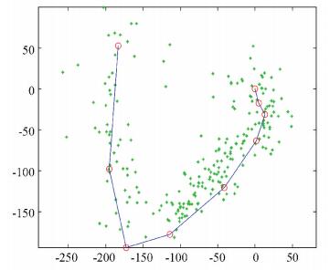
The landmarks, selected way points and the experiment result are shown in Fig. 8 and Fig. 9. In Fig. 8, the red circles connected by blue lines sequentially are the selected way points and the green points are the landmarks. It is worth noting that the blue line is not the actual movement path of the robot, just for a better display.
|
Figure 9 Landmarks and selected way points |
The experiment was run on the same computer as the simulation section, and the configuration of the compared SLAM algorithms was the same except the size of particles.
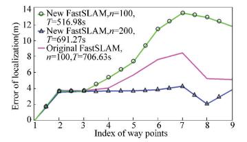
As shown in the Fig. 10, the experiment result was similar to the simulation result, where the time consumption was shown in the tag bar. The error of non-intact FastSLAM was bigger than the original FastSLAM under the same size of particles. However, the time consumption of the presented algorithm (516.98 s) was smaller than the original algorithm (706.63 s) by 26.9%. After doubling the particle size of the non-intact FastSLAM, the error became smaller than the original one by 10%-60%. In addition, time consumption (691.27 s) was still less than the original algorithm.
|
Figure 10 Localization error of experiment |
6 Conclusions
A RBPF algorithm with non-intact particle data has been proposed in this paper. With this algorithm, the idea of differentiating the particles data in the particle filter has been proposed. From the simulation and the experiment results, it can be seen that compared with the original FastSLAM, the efficiency of the presented algorithm has been improved considerably on the decline of mapping accuracy in a certain degree under the same size of particles. And the computational efficiency is more obvious with the increment of particle size. However, by increasing the size of particles, the accuracy can be better while the time consumption is also less than the original one.
In the meanwhile, compared with original FastSLAM algorithm, the proposed algorithm has a smaller data space occupation because the number of individual maps is reduced. In addition, this study focuses on RBPF actually rather than FastSLAM. The RBPF has wide application in many engineering problems besides SLAM. Therefore, other applications based on RBPF may benefit from this study.
In the future, the following work need to be studied:
(A) Verification by the theoretical derivation;
(B) Satisfactory tuning method of proposed parameters in the algorithm.
| [1] |
Thrun S, Fox D, Burgard W, et al. Robust monte carlo localization for mobile robots. Artificial Intelligence, 2001, 128(1-2): 99-141. DOI:10.1016/S0004-3702(01)00069-8 (  0) 0) |
| [2] |
Cadena C, Carlone L, Carrillo H, et al. Past, present, and future of simultaneous localization and mapping: Towards the robust-perception age. IEEE Transactions on Robotics, 2016, 32(6): 1309-1332. DOI:10.1109/TRO.2016.2624754 (  0) 0) |
| [3] |
Cox I J, Wilfong G T. Autonomous Robot Vehicles. New York: Springer-Verlag, 1990.
(  0) 0) |
| [4] |
Li J S, Li Y Q, Zhou D. Analysis of the consistency of EKF-based SLAM. Computer Simulation, 2008, 25(6): 155-160. (  0) 0) |
| [5] |
Doucet A, de Freitas N, Murphy K P, et al. Rao-blackwellized particle filtering for dynamic Bayesian networks. Proceedings of the 16th Annual Conference on Uncertainty in Artificial Intelligence (UAI). San Francisco, CA: Morgan Kaufmann Publishers Inc., 2000.171-176.
(  0) 0) |
| [6] |
Grisetti G, Stachniss C, Burgard W. Improved techniques for grid mapping with Rao-Blackwellized particle filters. IEEE Transactions on Robotics, 2007, 23(1): 34-46. DOI:10.1109/TRO.2006.889486 (  0) 0) |
| [7] |
Montemerlo M, Thrun S, Koller D, et al. FastSLAM: A factored solution to the simultaneous localization and mapping problem.Proceedings of the AAAI National Conference on Artificial Intelligence. Reston, VA: AAAI, 2002. 593-598.
(  0) 0) |
| [8] |
Li X Z, Ju H H. A simultaneous localization and map-building method for lunar rover based on particle filter. Journal of Astronautics, 2009, 30(5): 1891-1895. DOI:10.3873/j.issn.1000-1328.2009.05.024 (  0) 0) |
| [9] |
Pei F J, Li H Y, Cheng Y H. An improved FastSLAM system based on distributed structure for autonomous robot navigation. Journal of Sensors, 2014, 45(6): 289-298. DOI:10.1155/2014/456289 (  0) 0) |
| [10] |
Song Y, Li Q L, Kang Y F, et al. CFastSLAM: a new Jacobian free solution to SLAM problem. 2012 IEEE International Conference on Robotics and Automation, Piscataway:IEEE, 2012, 3063-3068. DOI:10.1109/ICRA.2012.6224822 (  0) 0) |
| [11] |
Song Y, Li Q L, Kang Y F, et al. Square-root Cubature FastSLAM algorithm for mobile robot simultaneous localization and mapping. 2012 IEEE International Conference on Mechatronics and Automation. Piscataway:IEEE, 2012, 1162-1167. DOI:10.1109/ICMA.2012.6283415 (  0) 0) |
| [12] |
Mur-Artal R, Tard'os J D. ORB-SLAM2: An open-source SLAM system for monocular, stereo and RGB-D cameras. IEEE Transactions on Robotics, 2017, 33(5): 1255-1262. DOI:10.1109/TRO.2017.2705103 (  0) 0) |
| [13] |
Engel J, Schöps, T Cremers D. LSD-SLAM: Large-scale direct monocular SLAM. European Conference on Computer Vision: ECCV 2014, Computer Science. Berlin: Springer, 2014, 8690: 834-849.
(  0) 0) |
| [14] |
Strasdat H, Montiel J M M, Davison A J. Visual SLAM: why filter?. Image and Vision Computing, 2012, 30(2): 65-77. DOI:10.1016/j.imavis.2012.02.009 (  0) 0) |
| [15] |
Thrun S, Burgard W, Fox D. Probabilistic Robotic. Cambridge MA: MIT Press, 2005.
(  0) 0) |
| [16] |
Stachniss C. Robotic Mapping and Exploration. New York: Springer-Verlag, 2009.
(  0) 0) |
| [17] |
Cai Z X, He H G, Chen H. Mobile Robot Navigation Control Theory and Methods in Unknown Environment. Beijing: Science Press, 2009.
(  0) 0) |
| [18] |
de Melo Neto A, Rosa P F F, de Oliveira T E A, et al. Efficiency of the visual FastSLAM technique with a common feature map for two vehicles in the integrated exploration of an indoor environment. Journal of Control, Automation and Electrical Systems, 2013, 24(4): 450-469. DOI:10.1007/s40313-013-0041-2 (  0) 0) |
| [19] |
Silveira Vidal F, Ferreira Rosa P F, de Melo Neto A, et al. Cooperating robots for mapping tasks with a multilayer perceptron. Poceedings of the 39th Annual Conference of the IEEE Industrial Electronics Society. Piscataway: IEEE, 2013. 4073-4078. DOI: 10.1109/IECON.2013.6699788.
(  0) 0) |
| [20] |
Yang C K, Hsu C C, Wang Y T. Computationally efficient algorithm for simultaneous localization and mapping (SLAM). Proceedings of the 2013 10th IEEE International Conference on Networking, Sensing and Control. Piscataway: IEEE, 2013. 328-332. DOI: 10.1109/ICNSC.2013.6548759.
(  0) 0) |
| [21] |
Montemerlo M, Thrun S. FastSLAM: A Scalable Method for the Simultaneous Localization and Mapping Problem in Robotics. New York: Springer-Verlag, 2007.
(  0) 0) |
 2018, Vol. 25


