2. School of Electrical Engineering and Information, Northeast Petroleum University, Daqing 163318, Heilongjiang, China
Under the influences of both the geological environment and acquisition conditions, seismic data is prone to dead traces, insufficient spatial sampling, and noise introduction, while demands for the integrity and regularity of seismic data are high in the subsequent processing and interpretation, hence the recovery of undersampled data is an extremely critical problem. The traditional seismic data recovery method[1-2] is restricted by the Nyquist sampling theory, which rules that the sampling frequency is at least two times of the highest frequency of the signal, otherwise it is very easy to result in aliased, consequently affecting the quality of recovery. Recently, the theory of compressed sensing as proposed by Candès[3] and Donoho[4] claims that under certain conditions, signals to be sampled at sub-Nyquist rates via linear projection onto a random basis while still could be accurately recovered[5-7], which provides a new idea for the problem of seismic data recovery. Curvelet transformation[8] with the significant advantages of directional sensitivity and anisotropy, can effectively represent multiple directional events, further making use of sparse seismic data, which has been used extensively in seismic data processing[9-10]. Herrmann and Hennenfent in Ref.[11] applied compressed sensing to the problem of seismic data recovery in the curvelet domain for the first time, further the curvelet-based recovery by the sparsity-promoting inversion[12] method was proposed the solving the sparse optimization problem. Shahidi et al. [13] used the cooling iterative threshold method to solve the L1 norm minimization problem in seismic data recovery, with the prior knowledge that the seismic data could be sparsely represented in the curvelet domain. The above solutions of the recovery problems depend critically on the seismic data's sparsity in curvelet transformed domain, as well as the simple and effective soft threshold in the iterative shrinkage process based on compressed sensing. But the soft threshold method inherently assumes that all the curvelet coefficients are completely independent, hence the classical soft shrinkage function is used to determine the significances of all curvelet coefficients in each iteration, and however the dependencies between curvelet coefficients are entirely ignored. Naghizadeh[14] also reported a curvelet transform interpolation scheme that the curvelet coefficients were divided into two groups of scales: alias-free (coarse) scalse and alias-contaminated (high) scales, then the alias-free curvelet coefficients were upscaled to estimate a mask function that was used to constrain the inversion of the alias-contaminated scale coefficients, but the strong dependencies between a coefficient and its parent were not captured as well. Bayesian estimation techniques were widely used in the field of data processing[15-17], moreover Sendur[18] proposed the bivariate shrinkage functions using the bayesian maximum posterior probability estimation to denoise natural image in wavelet domain, which yielded performance superior to soft shrinkage function, in that it exploited the statistical dependencies of neighborhood and parent-child.
Amongst all these methods, it was observed that the dependencies between curvelet coefficients should be taken into account to calculate the shrinkage function instead of the simple soft shrinkage function, when the iterative shrinkage process was used to recover the seismic data based on compressed sensing. Inspired by Ref.[18], we focus on the parent-child curvelet coefficients dependencies of seismic data with the Bayesian estimation techniques in order to address this issue. Our contribution lies in that we model the joint parent-child distribution of curvelet coefficients, furthermore obtaining the bivariate shrinkage function based on bayesian maximum posterior probability estimation, in order to predict the true coefficients of observed seismic data (undersampled), and then the distribution characteristics of the finest-scale and neighbor curvelet coefficients of seismic data are used to determine the parameters, finally the Landweber iterative shrinkage algorithm is used in the recovery process. In experimental simulations, we find that the proposed algorithm usually matches or exceeds PSNR performance of the soft shrinkage function, and maintains the texture details better in the events of the recovery of seismic data.
2 Principle of Seismic Data Recovery Based on Compressed SensingSet
| $ \mathit{\boldsymbol{y}} = \mathit{\boldsymbol{Rx}} $ | (1) |
where R is a randomly sampling matrix, which is used to extract y from x. Though the Eq. (1) is a set of underdetermined equations, in which x can not be solved according to y. But as we all known that the coefficients of seismic data in the curvelet domain is sparse, let α as the curvelet coefficients of the seismic data, C as the curvelet transform, and CT the inverse curvelet transform, then the Eq.(1) can be written as Eq.(2).
| $ \mathit{\boldsymbol{y}} = \mathit{\boldsymbol{Rx}} = \mathit{\boldsymbol{R}}{\mathit{\boldsymbol{C}}^{\rm{T}}}\mathit{\boldsymbol{\alpha }} = {\mathit{\boldsymbol{A}}^{CS}}\mathit{\boldsymbol{\alpha }} $ | (2) |
According to the theory of compressed sensing, if the sensing matrix ACS meets the Isometric Property Restricted (RIP)[19], the fully-sampled seismic data could be recovered by the
| $ \min {\left\| \mathit{\boldsymbol{\alpha }} \right\|_1}{\rm{s}}.{\rm{t}}.\;{\mathit{\boldsymbol{A}}^{CS}}\mathit{\boldsymbol{\alpha }} = \mathit{\boldsymbol{R}}{\mathit{\boldsymbol{C}}^{\rm{T}}}\mathit{\boldsymbol{\alpha }} = \mathit{\boldsymbol{y}} $ | (3) |
As α is sparse, it can be solved by the sparsity-promoting inversion algorithm of the formula (4).
| $ \mathit{\boldsymbol{\hat \alpha }} = \arg \min \frac{1}{2}\left\| {\mathit{\boldsymbol{y}} - {\mathit{\boldsymbol{A}}^{CS}}\mathit{\boldsymbol{\alpha }}} \right\|_2^2 + \beta {\left\| \mathit{\boldsymbol{\alpha }} \right\|_1} $ | (4) |
where β is the balance factor,
| $ {\mathit{\boldsymbol{\alpha }}^{\left( {k + 1} \right)}} = T\left( {{\mathit{\boldsymbol{\alpha }}^{\left( k \right)}} + {\mathit{\boldsymbol{R}}^{\rm{T}}}\left( {\mathit{\boldsymbol{y}} - \mathit{\boldsymbol{R}}{\mathit{\boldsymbol{\alpha }}^{\left( k \right)}}} \right)} \right) $ | (5) |
| $ T\left( \mathit{\boldsymbol{\alpha }} \right) = \left\{ {\begin{array}{*{20}{c}} \begin{array}{l} \mathit{\boldsymbol{\alpha }},\\ 0, \end{array}&\begin{array}{l} \left| \mathit{\boldsymbol{\alpha }} \right| \ge \lambda \\ {\rm{else}} \end{array} \end{array}} \right. $ | (6) |
As the threshold λ is gradually decreased in cooling threshold method of each iteration, the vector proximate to y = Rx super plane can be located, corresponding to
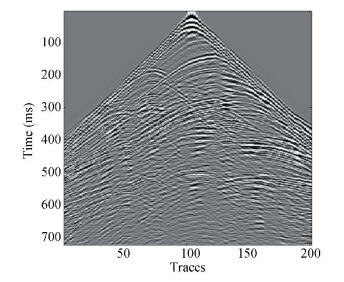
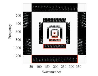
A curvelet is a geometric and directional wavelet, which has anisotropic needle-shape elements, and makes an optimal sparse representation of signals with continuities along smooth curves. Where the curvelet basis and signal edges are in the same direction, it will produce large coefficiencies; otherwise the random noise usually corresponds to small coefficients in the cruvelet domain. Just for this reason the curvelet is more appropriate for the two-dimensional signals with curves and edges, and it also will achieve higher approximation accuracy and better sparse representation. The seismic data is gathered in the process of artificial seismic exploration, thus they are of a huge dynamic range with a wealth of low-intermediate frequency information, in addition problems such as an insufficient sampling rate and low accuracy often occur due to the effect of technical, and/or geological conditions, and the effects of human action. However the wave fronts in the seismic data are usually composed of curved lines, which are very similar to the curve shape primitives of curvelet transform as shown in Fig. 1. Therefore the curvelet transform has extensively been used to approximate the wave front curve in seismic data, as aforementioned, the stronger events directivity are, the greater curvelet coefficients, and vice versa. The curvelet coefficients of Fig. 1 as shown in Fig. 2(by 5 scales decomposition). The white subbands are the isolated strips of curvelet coefficients, and they are not the real coefficients, just enough to satisfy the needs of the display. The black subbands are the curvelet coefficients regions, in which the brighter the pixels are in these regions, the greater the value of the coefficients, and conversely the smaller. The coefficients in the red boxes represents the same direction of different scales, where the scales vary from coarse to fine as the regions move from the center to outwards. Take the regions surround by red boxes as an example, according to the multi-scale feature of curvelet coefficients, the parent-child relationship of curvelet coefficients are established from above to below, as shown in Fig. 3(For the purpose of convenient observation, the coefficients of all directions are mapped in the same size). The distribution of current coefficients are very similar to the parents, if the paternal coefficients are important, the current coefficients are likely to be important, so it can be used to estimate the importance of current coefficients.
|
Figure 1 Fully-sampled Seismic data |
|
Figure 2 Curvelet coefficients |

|
Figure 3 Parent-child relationship of curvelet coefficients |
Usually, the noise affected by random missing traces are corresponding to the relatively small coefficients in the curvelet domain, where the soft shrinkage function that main idea is to retain from all coefficients larger than the threshold, and further set all other coefficients to zero, is effectively promoting sparsity under the relatively high sampling rate, and it will gain a better recovery effect. However when the sampling rate is becomes lower, the curved feature of events in observed seismic data are destroyed, as a result, without the obvious directional information, there will be a large number of small curvelet coefficients. Furthermore, the true signal coefficients and noise coefficients can not be distinguished, if we determine the significance of coefficients only based on amplitude like the soft shrinkage function, consequently it will cause recovery problems of due to discontinuous events or serious blocking artifacts.
4 Multi-Scale Analysis of Seismic Data in Curvelet Domain 4.1 Curvelet Bivariate Shrinkage FunctionThere are strong correlations among the curvelet coefficients which are between adjacent scales, so it is possible to predict the true value of the observed seismic data, according to the respective joint parent-child curvelet coefficients distribution models of fully-sampled seismic data and noise signal, coupled with the Bayesian maximum a posteriori estimator.
Set γ is the curvelet coefficient of observed seismic data, w is the fully-sampled seismic data curvelet coefficient, and ε is the noise signal curvelet coefficient, so there is: γ=w+ε.
According to Bayesian theory, under the condition that γ is known, the maximum posteriori probability is estimated as the formula (7).
| $ \hat w\left( \gamma \right) = \arg \mathop {\max }\limits_w {p_{w\left| \gamma \right.}}\left( {w\left| \gamma \right.} \right) $ | (7) |
The formula (8) is obtained by using Bayesian rule:
| $ \begin{array}{*{20}{c}} {\hat w\left( \gamma \right) = \arg \mathop {\max }\limits_w \left[ {{p_{\left( {\gamma \left| w \right.} \right.}}\left( {\gamma \left| w \right.} \right) \cdot {p_w}\left( w \right)} \right] = }\\ {\arg \mathop {\max }\limits_w \left[ {{p_\varepsilon }\left( {\gamma - w} \right) \cdot {p_w}\left( w \right)} \right]} \end{array} $ | (8) |
It is equivalent to Eq.(9),
| $ \hat w\left( \gamma \right) = \arg \mathop {\max }\limits_w \left[ {\log \left( {{p_\varepsilon }\left( {\gamma - w} \right)} \right) + \log \left( {{p_w}\left( w \right)} \right)} \right] $ | (9) |
where pw is the probability distribution function of curvelet coefficients of full-sampled seismic data, pε is the probability distribution function of noise signal curvelet coefficients. Let γ2 represent the parent of γ1. (γ2 is the curvelet coefficient at the same direction as γ1, but at the adjacent coarser scale), Similarly let w2 represent the parent of w1, and ε2 represent the parent of ε1, so one can get w=(w1, w2), γ=(γ1, γ2), ε=(ε1, ε2).
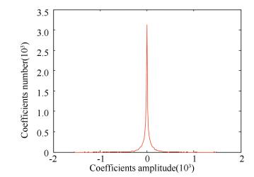
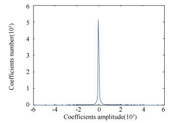
In this paper, the respective distributions in various scales of curvelet coefficients are obtained according to a lot of experiments, as a result the former is shown as Fig. 4, which is approximate to the Gaussian distribution, while the latter is shown as Fig. 5, which is approximate to the Laplasse distribution.
|
Figure 4 Distribution of noise |
|
Figure 5 Distribution of fully-sampled Seismic data |
We model the noise caused by missing traces in each scale curvelet domain by a zero mean Gaussian distribution, so the joint parent-child coefficients probability distribution function can be defined as Eq.(10).
| $ {p_\varepsilon }\left( \varepsilon \right) = \frac{1}{{2{\rm{ \mathsf{ π} }}\sigma _\varepsilon ^2}}\exp \left( { - \frac{{\varepsilon _1^2 + \varepsilon _2^2}}{{2\sigma _\varepsilon ^2}}} \right) $ | (10) |
where σε is the mean variance of curvelet coefficients of noise signal.
In that the curvelet coefficients of the fully-sampled seismic data are more approximate to the Laplasse distribution, the joint probability distribution function of the parent-child coefficients can be defined as the formula (11):
| $ {p_w}\left( w \right) = \frac{1}{{2{\rm{ \mathsf{ π} }}{\sigma ^2}}}\exp \left( { - \frac{{\sqrt 2 }}{\sigma }\left( {\left| {{w_1}} \right| + \left| {{w_2}} \right|} \right)} \right) $ | (11) |
where σ is the mean variance of curvelet coefficients of the fully-sampled seismic data.
Bring formula (10), (11) into (9), obtained formula (12):
| $ \begin{array}{l} \hat w\left( \gamma \right) = \arg \mathop {\max }\limits_w \left[ { - \frac{{{{\left( {{\gamma _1} - {w_1}} \right)}^2}}}{{2\sigma _\varepsilon ^2}} - \frac{{{{\left( {{\gamma _2} - {w_2}} \right)}^2}}}{{2\sigma _\varepsilon ^2}} + } \right.\\ \;\;\;\;\;\;\;\;\left. {\log \left( {{p_w}\left( w \right)} \right)} \right] \end{array} $ | (12) |
If pw(w) is convex and differentiable, after finishing one can get the formula (13):
| $ {{\hat w}_1} = \frac{{{{\left( {\sqrt {\gamma _1^2 + \gamma _2^2} - \frac{{\sqrt 3 \sigma _\varepsilon ^2}}{\sigma }} \right)}_ + }}}{{\sqrt {\gamma _1^2 + \gamma _2^2} }} \cdot {\gamma _1} $ | (13) |
where (g)+=0, for g < 0, (g)+=g else, and it is the bivariate shrinkage function of curvelet coefficients but the final solution needs to predict the mean square variance of noise signal curvelet coefficients σε, and mean square variance of fully-sampled seismic data curvelet coefficients σ. Due to the curvelet coefficients of observed seismic data in finest-scales usually contain a large number of noise signal coefficients and few significant coefficients; we use the median of finest-scale coefficients as the σε estimated value. Besides the interscale dependencies, there are strong dependencies between the adjacent coefficients, then σ as the marginal variance of coefficient γ1 is estimated in a local 3 × 3 neighborhood surrounding γ1 in this paper. So far, the bivariate shrinkage function is finished, which illustrates the effect of taking into account the parent-child dependencies, moreover shows that the determination of curvelet coefficients significance is no longer solely according to magnitude of the current coefficients, but the parent coefficients and neighborhood coefficients, the smaller the parent value, the greater the shrinkage for current coefficient, particularly if parent γ2 is 0, we get the soft shrinkage function
In the recovery process based on compressed sensing, we use the Landweber iterative algorithm with the iterative shrinkage strategy, then the bivariate shrinkage function is used to promote sparsity in each iteration such as Eq.(14):
| $ \tilde T\left( {\gamma _i^{\left( {k + 1} \right)}} \right) = \left\{ \begin{array}{l} \hat w_i^{\left( {k + 1} \right)},\sqrt {\gamma _i^2 + \gamma _{i - 1}^2} > \frac{{\sqrt 3 \sigma _\varepsilon ^2}}{\sigma }\\ 0,\;\;\;\;\;\;\;\;\;{\rm{else}} \end{array} \right. $ | (14) |
where γi(k+1) represents the i scale curvelet coefficients of the observed seismic data in the k+1 iteration, while
The proposed algorithm of seismic data recovery based on compressed sensing is described as follows:
Algorithm 1 The seismic data recovery algorithm with curvelet bivariate shrinkage function based on compressed sensing.
Algorithm steps:
Input: Given the iteration stop parameters τ, the maximum number of iterations K, the seismic data observation matrix R, observed seismic data y.
Output: Recovery of seismic data x.
1) Initialization: Iterative counter k=1, curvelet transform operator C, number of transform scales s, the curvelet bivariate shrinkage function
2) while (k≤K)
for i=2 to s
end for
if (‖ x(k+1)- x(k)‖2≤ τ)
break;
end if
end while
return
In order to validate the feasibility and effectiveness of the proposed algorithm, we compare the proposed algorithm with the existing algorithms by using synthetic seismic data and the Marmousi model seismic data as examples. Our approach was that first we got both of the fully-sampled seismic data sets, and then they are extracted by randomly sampling matrix to generate the observed seismic data (with random missing traces), finally the proposed algorithm is used to recover the observed seismic data. The objective measurement of the recovery data is based on the peak signal to noise ratio (PSNR), as shown in the formula (15):
| $ {P_{SNR}} = 10 \times {\log _{10}}\frac{{\max {{\left( \mathit{\boldsymbol{f}} \right)}^2}}}{{{\rm{MSE}}}} $ | (15) |
where f is the vector of the fully-sampled seismic data, MSE is the mean square error of f and the vector of the recovered seismic data.
5.1 Experimental Analysis of Synthetic Seismic DataThe partial single shot seismic synthetic records is shown in Fig. 6(a) and the observed data under 70% sampling rate is shown in Fig. 6(b). The Fig. 6(c) shows the recovery effect of soft shrinkage function iterative algorithm, and the Fig. 6(d) shows the recovery effect of proposed algorithm, as we can see the events in elliptical selection area of Fig. 6(c) are fuzzy and have an obvious block effect, while the corresponding region in Fig. 6(d) is relatively continuous and smooth. Fig. 6(e) illustrates the comparison of PSNR evolution curves with respect to an iteration number with an under 70% sampling rate, with the increasing number of iterations, the PSNR of two algorithms are gradually improved, but the proposed algorithm is first to achieve convergence, and the convergence value is higher than that of the soft shrinkage function algorithm. Fig. 6(f) illustrates the PSNR comparison of the two algorithms under different sampling rates, and we can see that the proposed algorithm in different sampling rates gains higher PSNR than the soft shrinkage function algorithm.

|
Figure 6 The experiment with synthetic data |
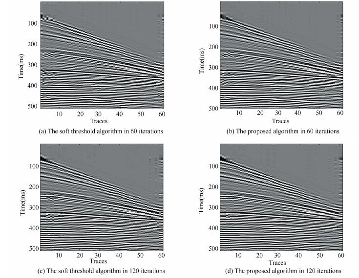
Fig. 7 shows the effect of the soft threshold algorithm and the proposed algorithm in 60, and 120 iterations. It can be seen that under the same number of iterations, the proposed algorithm can maintain events better, and the curve feature is more smooth and continuous.
|
Figure 7 The experiment of different number of iterations |
5.2 Experimental Analysis of the Marmousi Model
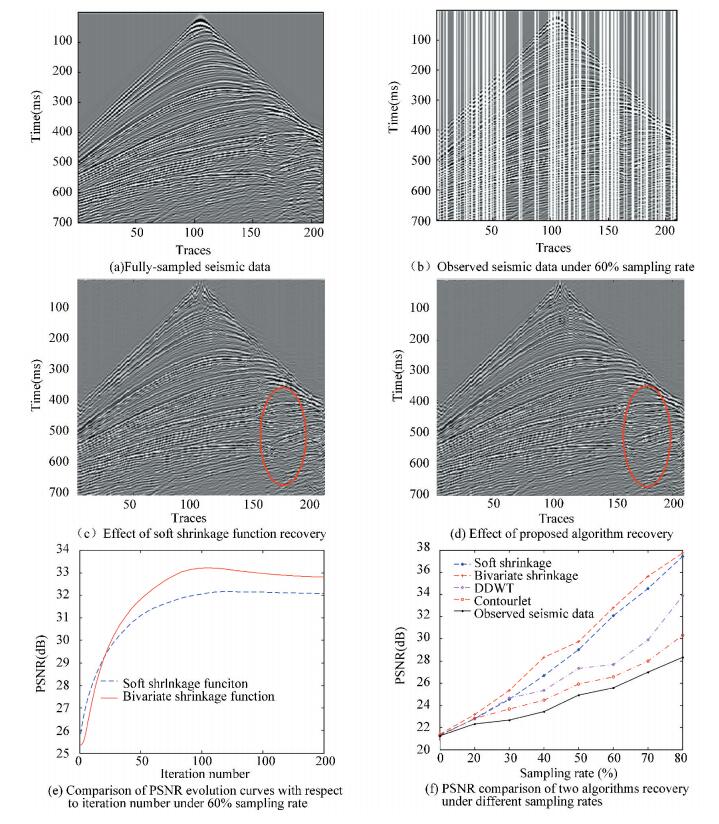
The Marmousi model is used to test the proposed algorithm further, the fully-sampled seismic data is shown in Fig. 8(a), and the observed data with an under 60% sampling rate is shown in Fig. 8(b). The Fig. 8(c) shows the recovery effect of the soft shrinkage function iterative algorithm, and the Fig. 8(d) shows the recovery effect of the proposed algorithm, as we can see that the events in elliptical selection area of Fig. 8(c) have a more prominent block effect, while the corresponding region in Fig. 8(d) is relatively smooth. Fig. 8(e) illustrates the comparison of PSNR evolution curves with respect to an iteration number under with a 60% sampling rate, with the increase in the number of iterations, we can see that the PSNR value of the proposed algorithm is lower than that of the former at the beginning, but after 20 iterations, the convergence speed is apparently accelerated, eventually converging to the higher PSNR. Because the dual tree complex wavelet transformation (DDWT) and contourlet transformation have a good ability for sparse representation with texture and contour information, Fig. 8(f) illustrates the PSNR comparison of four algorithms under different sampling rates, it shows that the reconstruction effect of curvelet transformation is higher than that of the DDWT and contourlet, and the reconstruction effect of the bivariate threshold algorithm being better than that of the soft threshold reconstruction algorithm in different sampling rates. The above experiments have proved that the proposed algorithm is more effective and adaptable.
|
Figure 8 The experiment with marmousi model data |
Table 1 demonstrates the run time comparison of the proposed algorithm with the soft threshold algorithm, DDWT and contourlet in the different sampling rates, under the 200 iterations. In the same sampling rate, and the run time of the proposed algorithm is higher than that of the soft threshold algorithm for 20-50 s, because in each iteration of the threshold processing, the threshold is fixed in soft threshold algorithm, thus it just needs to compare the value of the current coefficients with the threshold, while in the proposed algorithm, it needs to not only to search for parent coefficients of current coefficients, but also generate the respective thresholds through the variance of neighborhood, and therefore it increases the computation requirements. As the efficiency of DDWT and contourlet transformation is higher than the curvelet transformation, the running time is relatively short.
| Table 1 Comparison of run time under different sampling rate |
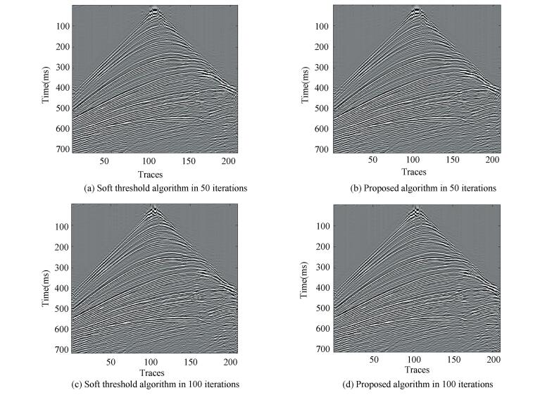
Fig. 9 shows the recovered effect of the soft threshold algorithm and the proposed algorithm in 50, 100 iterations. It can be seen that with the increasing of the iterative number, the subjective effect of the two algorithm is enhanced, and the quality of the two recovered images is not so far different in the smooth region, but the reconstruction effect of the proposed algorithm is better than that of the former in the complex region of the events.
|
Figure 9 The experiment of different number of iterations |
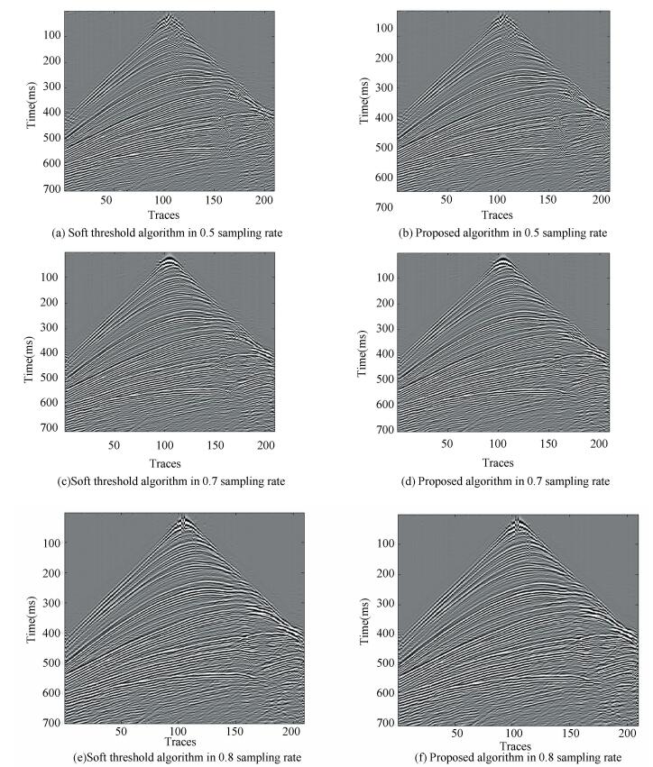
Fig. 10 illustrates the comparison of the recovered results between the soft threshold algorithm and the proposed algorithm, the two algorithms show some fuzzy phenomena at sampling rates of 0.5, 0.7 and 0.8. When the sampling rate is 0.5, the effect of the reconstructions of the complex region of the events. This is because the unified threshold processing is adopted to all scales in the soft threshold algorithm, while the proposed algorithm employs the correlation of the curvelet coefficients, thus the latter subjective effect is improved. With an increasing of sampling rate, such as the sampling rates of 0.7, 0.8, the advantages of the proposed algorithm in this paper are more obvious.
|
Figure 10 Experiment of different sampling rates |
6 Conclusions
In the idea of the compressed sensing recovery coupled with the iterative shrinkage method based on curvelet transform, the recovery algorithm using the curvelet bivariate shrinkage function is proposed. We first model the joint distribution of parent-child curvelet coefficients of fully-sampled seismic data by the Laplasse distribution, and the noise signal by zero mean Gauss distribution, and then the curvelet bivariate shrinkage function based on Bayesian maximum posteriori estimation is obtained. Furthermore, the distribution of finest-scale coefficients and the interscale dependencies are exploited to estimate the parameters of the curvelet bivariate shrinkage function. Finally, the Landweber iterative algorithm is used in the recovery process. The experiments on the synthetic and Marmousi model seismic data prove that the proposed algorithm can obtain higher recovery PSNR and has a better effect in maintaining the texture than the existing algorithms.
| [1] |
Spitz S. Seismic trace interpolation in F-X domain. Geophysics, 1991, 56(6): 785-794. DOI:10.1190/1.1443096 (  1) 1) |
| [2] |
Ronen J. Wave-equation trace interpolation. Geophysics, 2012, 52(7): 973-984. DOI:10.1190/1.1442366 (  1) 1) |
| [3] |
Candes E J, Romberg J, Tao T. Robust uncertainty principles: exact signal reconstruction from highly incomplete frequency information. IEEE Transactions on Information Theory, 2006, 52(2): 489-509. DOI:10.1109/TIT.2005.862083 (  1) 1) |
| [4] |
Donoho D L. Compressed sensing. IEEE Transactions on Information Theory, 2006, 52(4): 1289-1306. DOI:10.1109/TIT.2006.871582 (  1) 1) |
| [5] |
Tropp J A, Gilbert A C. Signal recovery from random measurements via orthogonal matching pursuit. IEEE Transactions on Information Theory, 2007, 53(12): 4655-4666. DOI:10.1109/TIT.2007.909108 (  1) 1) |
| [6] |
Needell D, Vershynin R. Signal recovery from incomplete and inaccurate measurements via regularized orthogonal matching pursuit. IEEE Journal of Selected Topics in Signal Processing, 2007, 4(2): 310-316. DOI:10.1109/JSTSP.2010.2042412 (  1) 1) |
| [7] |
Figueiredo M A T, Nowak R D, Wright S J. Gradient projection for sparse reconstruction: Application to compressed sensing and other inverse problems. IEEE Journal of Selected Topics in Signal Processing, 2008, 1(4): 586-597. DOI:10.1109/JSTSP.2007.910281 (  1) 1) |
| [8] |
Candès E J, Donoho D L. New tight frames of curvelets and optimal representations of objects with smooth singularities. Communications on Pure & Applied Mathematics, 2004, 57(2): 219-266. DOI:10.1002/cpa.10116 (  1) 1) |
| [9] |
Herrmann F J, Wang D, Hennenfent G, et al. Curvelet-based seismic data processing: A multiscale and nonlinear approach. Geophysics, 2008, 73(1): 2220-2237. DOI:10.1190/1.2799517 (  1) 1) |
| [10] |
Ma J, Plonka G. A review of curvelets and recent applications. IEEE Signal Processing Magazine, 2010, 27(2): 118-133. DOI:10.1109/MSP.2009.935453 (  1) 1) |
| [11] |
Herrmann F J, Hennenfent G. Non-parametric seismic data recovery with curvelet frames. Geophysical Journal International, 2008, 173(1): 233-248. DOI:10.1111/j.1365-246X.2007.03698.x (  1) 1) |
| [12] |
Daubechies I, Defrise M, de Mol C. An iterative thresholding algorithm for linear inverse problems with a sparsity constraint. Communications on Pure & Applied Mathematics, 2004, 57(11): 1413-1457. DOI:10.1002/cpa.20042 (  1) 1) |
| [13] |
Shahidi R, Tang G, Ma J, et al. Application of randomized sampling schemes to curvelet-based sparsity-promoting seismic data recovery. Geophysical Prospecting, 2013, 61(5): 973-997. DOI:10.1111/1365-2478.12050 (  1) 1) |
| [14] |
Naghizadeh M, Sacchi M D. Beyond alias hierarchical scale curvelet interpolation of regularly and irregularly sampled seismic data. Geophysics, 2010, 75(6): 189-202. DOI:10.1190/1.3509468 (  1) 1) |
| [15] |
Wang Yuhui, Wang Wei, Wu Qingxian. Winning probability estimation based on improved bradley-terry model and Bayesian network for aircraft carrier battle. Journal of Harbin Institute of Technology(New Series), 2017, 24(2): 39-44. DOI:10.11916/j.issn.1005-9113.15254 (  1) 1) |
| [16] |
Ding S, Wang L. A scheme of sEMG feature extraction for improving myoelectric pattern recognition. Journal of Harbin Institute of Technology(New Series), 2016, 23(2): 59-65. DOI:10.11916/j.issn.1005-9113.2016.02.009 (  1) 1) |
| [17] |
Afshari M, Lak F, Gholizadeh B. A new Bayesian wavelet thresholding estimator of nonparametric regression. Journal of Applied Statistics, 2016, 44(4): 1-18. DOI:10.1080/02664763.2016.1182130 (  1) 1) |
| [18] |
Sendur L, Selesnick I W. Bivariate shrinkage functions for wavelet-based denoising exploiting interscale dependency. IEEE Transactions on Signal Processing, 2002, 50(11): 2744-2756. DOI:10.1109/TSP.2002.804091 (  2) 2) |
| [19] |
Candès E J. The restricted isometry property and its implications for compressed sensing. Comptes Rendus Mathematique, 2008, 346(9-10): 589-592. DOI:10.1016/j.crma.2008.03.014 (  1) 1) |
 2018, Vol. 25


