For structural reliability problems, strength and stiffness reliabilities are generally considered. Besides, components of mechanisms should also meet the requirements of the performance reliability or the motion accuracy reliability (MAR).
Due to deterioration of performance parameters, mechanism systems cannot meet the performance requirements and even fail completely. The topic of mechanism reliability arises due to the possibility of disastrous failures of precision devices and the increase of the accuracy requirements[1-2]. Mechanism reliability is a comprehensive indicator that reflects the operating performance of the mechanisms used in industry. The MAR of mechanisms can be defined as the capacity of the motion error to remain within the allowable error for a specified period of using time under specified service conditions. Some studies have been conducted to investigate the MAR. A new methodology was proposed to evaluate the MAR of gear mechanisms with truncated random variables in Ref. [3]. Sun[4] proposed a general method for MAR analysis of mechanisms with clearance, involving random and epistemic uncertainty. Zhou[5] quantified the dynamic performance of planetary gear system to conduct risk assessment.Li[6] proposed a solving program of dynamic equations based on the Monte Carlo method considering uncertain parameters. Wang[7] proposed a Hybrid Dimension Reduction Method (HDRM) to solve the dependent joint clearance variables.
Space manipulator is a complex mechanical system affected by various design variables. Errors in manufacturing and installation are inescapable and usually follow a normal distribution according to the literature. Besides, numerous works have discussed the dynamic response of space mechanisms. Kakizaki et al.[8] established the dynamic model of space elastic manipulators with flexible link and joint clearance, and studied the effect of joint clearance and joint elasticity on system performance. Ting et al.[9] developed a new method for identifying the worst position and direction errors caused by joint clearance of manipulators. Yang et al.[10] established a nonlinear model of space manipulator joints considering time-varying stiffness and clearance, which are critical in precision manipulator systems.
Mechanism reliability research on multibody dynamics has been rarely reported[11]. Binaud et al.[12] used two nonconvex constrained quadratic programs to study the motion sensitivity of manipulators to joint clearances. Tsai and Lai[13] put forward a motion sensitivity analysis method considering joint clearance based on transmission quality. Lee and Gilmore[14] used the "effective link length" to determine the probabilistic characteristics of velocity and acceleration in a randomly defined planar pinned kinematic chain. Normally, in the research of motion reliability (MR) of manipulators, the first order second moment method (FOSM) and the Monte Carlo simulation (MCS) are mainly included in probability methods. Probability theory usually involves numerical approximations and assumptions of probability distributions. An interval algorithm is used to generate a closed interval which guarantees the real result. Interval analysis methods can track all possible solutions simultaneously and can be used to evaluate the time dependent MR of an organization at specific intervals[15].
Interval method is a non-probabilistic method, which is mainly used to deal with the uncertainty analysis of dynamic problems. Interval parameters are defined as uncertain but bounded parameters. It is usually easier to get the bounds of the interval parameters than to obtain the probability density functions (PDFs). Interval algorithm is one of the most effective methods to evaluate boundaries of interval polynomial functions (also called surrogate models)[16]. Viegas et al.[17] used the interval algorithm to consider the uncertainties of relevant parameters and carried out kinematics analysis for the parallel machine tool. Some other researchers used the interval methods, such as the Taylor series method[18], the vertex solution theorem[19], the combined parameter perturbation method and interval mathematics[20], and the combined modal superposition method and interval mathematics[21] to analyze simple perfect dynamics problems. Wei[22] presented an interval multi-dimensional harmonic balance method to solve the problem of the dynamic responses of parametrically excited systems under uncertainties and multi-frequency excitations. Wu et al.[21] presented a unified Chebyshev surrogate model to robustly assess geometrically nonlinear responses of engineering structures.
This paper mainly focuses on the MAR of manipulators with interval parameters. The object of this study is to develop a surrogate model by using Chebyshev inclusion function (CIF) to evaluate specific dynamic responses with interval parameters and to establish an interval reliability analysis model to obtain MAR. The CIF is proposed to evaluate the upper and lower bounds of the dynamic response of uncertain nonlinear dynamic systems. This inclusion function is also applicable to parameter systems, which is based upon the Chebyshev polynomial approximation and the interval arithmetic. It is a non-invasive method for parametric systems with uncertainties. The paper is organized as follows: in Section 2, the MAR of manipulators is defined and the probabilistic and the interval methods are introduced to estimate the MAR; in Section 3, the Chebyshev polynomial (CP) and the CIF are deduced to solve the dynamic equations of the system with interval parameters, where the CIF is used to generate the surrogate model for the system; in the last section, the proposed method is applied to an engineering structure and is proved to be efficient.
2 MAR of ManipulatorsWith the development of space manipulators towards high speed and high precision, MAR has become an important factor affecting the quality, life span, and reliability of products, thus drawing much attention. In the process of completing the task, the space manipulator must meet certain basic requirements such as precision, speed, and acceleration. Effect of each parameter on the performance of the system cannot be ignored.
Due to the restriction of test conditions and the unpredictability of operating conditions, such as vibration load, an accurate PDF with sufficient sample size could be constructed. However, some parameters (e.g., the angle of each joint) could merely be given the variation range for the lack of samples. Hence, using the interval model to evaluate the accuracy reliability is an approach with great engineering significance.
2.1 Probabilistic Reliability AnalysisSpace manipulator is an open-loop mechanism and the reliability of the positioning function is defined as the probability that the position and direction of the end effector are within the specified allowable area.
When S(X, t) is used to describe the dynamic parameter of the manipulator at some point t, X=[X1, X2, …, Xn] stands for the input parameter vector, and R(X, t) represents the threshold of the response.
The limit state function can be expressed as:
| $ g(\boldsymbol{X}, t)=R(\boldsymbol{X}, t)-S(\boldsymbol{X}, t) $ | (1) |
When g >0, the system is reliable; when g < 0, the system fails; and when g=0, the system is in a limit state. The MAR of the system could be defined as:
| $ R=Pr(g(\boldsymbol{X}, t)>0) $ | (2) |
Here, corresponding failure reliability is:
| $ P_{f}=1-R=1-{Pr}(g(\boldsymbol{X}, t)>0) $ | (3) |
| $ R = \mathit{\Phi }(\beta ) $ | (4) |
where β is reliability index and Φ(·) is standard normal distribution.
Therefore, the problem of solving the motion accuracy failure probability is converted to solving the probability when the limit state function is greater than zero. Such problem has been extensively studied and can be solved by first-order reliability methods, second-order reliability methods, and the like.
2.2 Interval Reliability AnalysisIn the above analysis, the input parameters are all random variables, while many of them cannot get an accurate PDF but a variation interval.
A real interval x=[a, b] is defined as a connected nonempty subset of real set R and according to the interval representation method. The interval can be expressed as follows:
| $ x \in x^{I} $ | (5) |
Any interval can be transformed to the expression of, such as:
| $ x=\frac{a+b}{2}+\frac{b-a}{2} \eta $ | (6) |
The system response and threshold intervals can be represented as:
| $ \left\{ {\begin{array}{*{20}{l}} {{R^I} = [\underline R, \bar R]}\\ {{S^I} = [\underline S, \bar S]} \end{array}} \right. $ | (7) |
where S and S are the upper and lower bounds of the system response, R and R the upper and lower bounds of the response thresholds, which can be obtained by interval operations.
Stress-strength intersects within a certain range of values, as shown in the shaded area in Fig. 1.

|
Fig.1 Non-probabilistic stress-strength interference model |
The stress and strength interval variables S∈SI, R∈RI are standardized as ηS∈[-1, 1] and ηR∈[-1, 1]. The state function changes into:
| $ G\left(\eta_{R}, \eta_{s}\right)=R^{R} \eta_{R}-S^{R} \eta_{S}+\left(R^{C}-S^{C}\right) $ | (8) |
where
| $ \begin{aligned} R^{C}=\frac{\underline R+\overline{R}}{2}, S^{C}=\frac{\underline S+\overline{S}}{2} \\ R^{R}=\frac{\overline{R}-\underline R}{2}, S^{R} &=\frac{\overline{S}-\underline S}{2} \end{aligned} $ |
The non-probabilistic reliability of the system response depends on the degree of stress-strength interference.
The two-dimensional normalized spatial interval stress intensity interference relationship is shown in Fig. 2.

|
Fig.2 Two-dimensional reliability model |
The variable region can be divided into two parts (i.e., a failure domain and a safe domain) by the limit state surface in the standard space. The probability that the generalized stress is greater than the generalized strength can be defined as the ratio of the area of the failure domain to the total area of the basic variable area[23]:
| $ P_{f}={Pr}\left(G\left(\eta_{R}, \eta_{S}\right)<0\right)=\frac{S_{\mathrm{Fail}}}{S_{\mathrm{Sum}}} $ | (9) |
When the threshold is a certain value, the reliability model degenerates to the ratio of lengths on several axes. The above method is also applicable to nonlinear systems. When the system contains more interval variables, the non-probabilistic failure rate becomes the ratio of the hypervolume of the failure domain to the total volume of the ultra-cuboid.
3 CIF Method for Interval ParametersIn many cases, the limit state function of the mechanism is often extremely complex and implicit. Using a simple function to approximate a continuous function over a given interval is the most effective way to study the uncertain dynamic response of manipulators. In this paper, the CIF method was used to fit the complex implicit kinematic function in order to obtain the bound of uncertain dynamic responses.
3.1 CP TheoryThe basic idea of the CP method is to approximate the original function using the sum of polynomials[24].
Considering the interval η=[1, 1], the range of the original function can be obtained from the CIF. For one-dimensional function with interval parameters, the pth order CIF is:
| $ [f](\eta ) = \frac{{{f_0}}}{2} + \sum\limits_{i = 1}^p {{f_i}} {C_i}(\eta ) = \frac{{{f_0}}}{2} + \sum\limits_{i = 1}^p {{f_i}} \cos i\theta $ | (10) |
where θ=arccos(η)∈[0, π] and Ci(η)=cosiθ denote the CP with order i. It is noted that C0(η)=1, Ci(η)=cosiθ=[-1, 1], and i≤1. Eq. (10) can thus be simplified as:
| $ \begin{aligned} ~[f](\eta) &=\frac{f_{0}}{2}+\sum\limits_{i=1}^{p} f_{i} C_{i}(\eta)=\frac{f_{0}}{2}+\\ &\left(\sum\limits_{i=1}^{p}\left|f_{i}\right|\right)[-1, 1] \end{aligned} $ | (11) |
The coefficient fi can be obtained by:
| $ {f_i} = \frac{2}{{p + 1}}\sum\limits_{j = 1}^{p + 1} f \left( {\cos {\theta _j}} \right)\cos i{\theta _j} $ | (12) |
where the interpolation points ηj are defined as the zeros of the CP with p+1:
| $ \eta_{j}=\cos \theta_{j}=\frac{2 j-1}{p+1} \cdot \frac{\pi}{2}, j=1, \cdots, p+1 $ | (13) |
With all the coefficients gained, the Chebyshev approximation polynomial of the original function can be obtained.
3.2 The CIF Method for Interval ParametersWu et al.[25] proposed the CIF to evaluate the bounds for an interval function and to control the overestimation in interval theory. The CIF is briefly introduced below and more information can be found in Ref.[26].
For multi-dimensional problems, the CIF can be expressed as:
| $ [f](\eta)=\sum\limits_{i_{1}=0}^{p} \ldots \sum\limits_{i_{m}=0}^{p}\left(\frac{1}{2}\right)^{l} f_{i_{1}, i_{2}, \cdots, i_{m}} C_{i_{1}, i_{2}, \cdots, i_{m}}(\eta) $ | (14) |
where l denotes the total number of constant items occurred in the subscripts i1, …, im, η=[-1, 1]m is an m-dimensional interval variable, and Ci1, i2, …, im(η) are the m-dimensional Chebyshev series, which are defined as the tensor product of each dimensional Chebyshev series.
| $ C_{i_{1}, \cdots, i_{n}}\left(\eta_{1}, \cdots, \eta_{m}\right)=\cos \left(i_{1} \theta_{1}\right) \cdots \cos \left(i_{m} \theta_{m}\right) $ | (15) |
The coefficients fi1, …, im can be calculated through the following equation:
| $ \begin{aligned} f_{i_{1}, \cdots i_{m}} &=\left(\frac{2}{p+1}\right)^{m} \sum\limits_{j_{1}=1}^{p+1} \ldots \sum\limits_{j_{m}=1}^{p+1} f\left(\cos \theta_{j_{1}}, \cdots, \cos \theta_{j_{m}}\right)\cdot \\ & \cos i_{1} \theta_{j_{1}} \cdots \cos i_{m} \theta_{j_{m}} \end{aligned} $ | (16) |
The more the dimensions are, the larger the computation cost. Therefore, the terms higher than pth order could be ignored and the format of the CIF is expressed as:
| $ \begin{aligned} ~[f](\eta) & \approx \sum\limits_{0 \leqslant i_{1}+\cdots+i_{m} \leqslant p}^{p}\left(\frac{1}{2}\right)^l f_{i_{1}, i_{2}, \cdots, i_{m}} C_{i_{1}, i_{2}, \cdots, i_{m}}(\eta)=\\ & \sum\limits_{i=0}^{N_{a}-1} y_{i} \psi_{i}(\eta) \end{aligned} $ | (17) |
where the remaining terms are equal to Nα=(m+p)!/(m!p!), the number of interpolation points is Ns=2Na, the coefficients (1/2)lfi1, i2, …, im correspond to yi, and Ci1, i2, …, im(η) correspond to ψi(η), respectively.
The Legendre polynomials in the transform matrix are required to change to the CP as:
| $ \boldsymbol{y}=\left(\boldsymbol{X}(\boldsymbol{\eta})^{\mathrm{T}} \boldsymbol{X}(\boldsymbol{\eta})\right)^{-1} \boldsymbol{X}(\boldsymbol{\eta})^{\mathrm{T}} \boldsymbol{f} $ | (18) |
where
| $ \boldsymbol{X}(\eta)=\left[ \begin{array}{ccc}{\psi_{0}\left(\eta_{1}\right)} & {\cdots} & {\psi_{N_{a}-1}\left(\eta_{1}\right)} \\ {\vdots} & {\vdots} & {\vdots} \\ {\psi_{0}\left(\eta_{N_{S}}\right)} & {\cdots} & {\psi_{N_{a}-1}\left(\eta_{N_{S}}\right)}\end{array}\right] $ | (19) |
where f denotes the model output vector at the interpolation points, and y=[y0, y1, …, yNa-1]T denotes the coefficients vector of the CP.
3.3 Sensitivity Analysis with the Interval UncertaintyInfluence of the variable on the non-probabilistic reliability index at the nominal value can be provided by the local sensitivity analysis of the non-probabilistic structure. In order to understand the effect of input variables over the entire range on output performance, it is necessary to study the global sensitivity of non-probabilistic structures. The global sensitivity analysis analyzes the influence of each parameter on the output of the model when all the design parameters of the system change at the same time and the influence of the interaction between the parameters on the model results. The effect of interval variables on the non-probabilistic reliability indices within their range of values is discussed in this section. Owing to the difficulty of solving the infinite norm, the global sensitivity based on the median-dispersion is studied here.
When the interval variable η takes the nominal value, the effect of the uncertainty of η on non-probabilistic reliability index would be eliminated. When the η changes within its ranges, the effect is still an interval value. The sensitivity can be defined as:
| $ \varepsilon_{i}=\frac{\beta_{\eta_{i}}^{R}}{\beta} $ | (20) |
where
Similarly, the sensitivity of the vector can be expressed as:
| $ {\varepsilon _{{j_1}, \cdots , {j_n}}} = \frac{{\beta _{{\eta _{j1}}, {\eta _{j2}}, \cdots , {\eta _{jn}}}^R}}{\beta } $ | (21) |
Where
| $ \begin{aligned} \beta_{\eta_{j 1}, \eta_{j 2}, \cdots, \eta_{j n}}^{R} &=\frac{1}{2}\left(\beta_{\eta_{j 1}, \eta_{j 2}, \cdots, \eta_{j n}}^{U}-\beta_{\eta_{j 1}, \eta_{j 2}, \cdots, \eta_{j n}}^{L}\right) \\ \beta_{\eta_{j 1}, \eta_{j 2}, \cdots, \eta_{j n}}^{C} &=\frac{1}{2}\left(\beta_{\eta_{j 1}, \eta_{j 2}, \cdots, \eta_{j n}}^{U}+\beta_{\eta_{j 1}, \eta_{j 2}, \cdots, \eta_{j n}}^{L}\right) \end{aligned} $ |
and
Discretization algorithm is presented to solve above sensitivity index for non-linear limit state function.
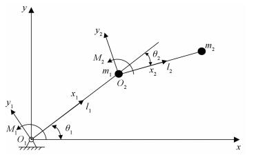
4 Case and DiscussionTo verify the feasibility of the proposed method, a two-link manipulator (see Fig. 3 and Fig. 4) was selected as the research object of this study.

|
Fig.3 Two-link manipulator in Adams |
|
Fig.4 Schematic of the two-link manipulator |
Because of the errors in manufacturing and assembly, the geometric variables of the manipulator can be regarded as interval variables.
Load inputs are affected by many factors such as manufacturing and assembly errors, elasticity of the gear-trains. Motion parameters of the two joints were also set as interval parameters. The basic variables are shown in Table 1, where M1 denotes the motion of the 1st joint, M2 denotes the motion of the 2nd joint, l1 denotes the length of the 1st link, and l2 denotes the length of the 2nd link. In addition, w and d correspond to the width and depth, respectively, t denotes the time.
| Table 1 Interval variables of the manipulator |
These components are produced separately and each motor works discretely. Therefore, it is reasonable to assume that these random variables are independent.
4.1 Kinematic Analysis of a Manipulator with Interval ParametersThe end coordinates are shown as follows:
| $ x_{\text { end }}=l_{1} \cos \theta_{1}+l_{2} \cos \left(\theta_{1}+\theta_{2}\right) $ | (22) |
| $ y_{\text { end }}=l_{1} \sin \theta_{1}+l_{2} \sin \left(\theta_{1}+\theta_{2}\right) $ | (23) |
Derivation of terminal coordinates to obtain terminal velocity equations are:
| $ \dot{x}_{\mathrm{end}}=-l_{1} w_{1} \sin \theta_{1}+l_{2}\left(w_{1}+w_{2}\right) \sin \left(\theta_{1}+\theta_{2}\right) $ | (24) |
| $ \dot{y}_{\text { end }}=-l_{1} w_{1} \cos \theta_{1}+l_{2}\left(w_{1}+w_{2}\right) \cos \left(\theta_{1}+\theta_{2}\right) $ | (25) |
where
| $ \left[ \begin{array}{c}{\dot{x}_{\mathrm{end}}} \\ {\dot{y}_{\mathrm{end}}}\end{array}\right]=\left[ \begin{array}{cc}{-l_{1} S_{1}-l_{2} S_{12}} & {-l_{2} S_{12}} \\ {l_{1} C_{1}+l_{2} C_{12}} & {l_{2} C_{12}}\end{array}\right] \left[ \begin{array}{c}{w_{1}} \\ {w_{2}}\end{array}\right] $ | (26) |
where
| $ \begin{array}{c}{S_{1}=\sin \theta_{1}, C_{1}=\cos \theta_{1}} \\ {S_{2}=\sin \theta_{2}, C_{2}=\cos \theta_{2}} \\ {S_{12}=\sin \left(\theta_{1}+\theta_{2}\right), C_{12}=\cos \left(\theta_{1}+\theta_{2}\right)}\end{array} $ |
In this study, the concerned manipulator is meshed by using a unified mesh of Absolute Nodal Coordinate Formulation (ANCF) because many types of finite elements of ANCF[27] have been applied to study the kinetics of deterministic multibody systems. The ANCF method establishes a constant mass matrix for multibody systems, which helps to improve computation efficiency. Based on the method of ANCF, the dynamic equations of the multibody system with uncorrelated random variables could be written as[28]:
| $ \left\{ {\begin{array}{*{20}{l}} {\mathit{\boldsymbol{M}}({\mathit{\boldsymbol{b}}})\mathit{\boldsymbol{\ddot q}} + {\mathit{\boldsymbol{F}}}({\mathit{\boldsymbol{q}}}, {\mathit{\boldsymbol{b}}}) + \mathit{\boldsymbol{ \boldsymbol{\varPhi} }}_q^{\rm{T}}({\mathit{\boldsymbol{q}}}, {\mathit{\boldsymbol{b}}}, t){\mathit{\boldsymbol{\lambda }}} = {\mathit{\boldsymbol{Q}}}({\mathit{\boldsymbol{q}}}, \mathit{\boldsymbol{\dot q}}, {\mathit{\boldsymbol{b}}})}\\ {\mathit{\boldsymbol{ \boldsymbol{\varPhi} }}({\mathit{\boldsymbol{q}}}, {\mathit{\boldsymbol{b}}}, \mathit{\boldsymbol{t}}) = 0} \end{array}} \right. $ | (27) |
where b denotes an n-dimensional vector of uncertain parameters, q denotes the vector of generalized coordinates, M denotes the constant mass matrix, F(q, b) denotes the vector of elastic forces, Φ(q, b, t) denotes the vector of the system constraint relations, Φq(q, b, t) denotes the derivative matrix of Φ(q, b, t) with respect to vector q, λ denotes the vector of Lagrange multipliers, and
In this work, the equivalent linear velocity of the end of the 2nd link was taken as the main performance parameter. The dynamic error was defined as the difference between the ideal output speed and the actual speed. The two-link rigid manipulator is studied in this paper. According to the load application (two torques) in this paper, the vibration excitation has little effect on the end of the link and it is of no significance to apply the vibration excitation. Thus the effect of frequency is not considered in this paper.
The system dynamic error can be expressed as a deterministic function of the vector ξ at any time t:
| $ \tilde{v}(\xi, t)=\phi\left(\xi_{1}, \xi_{2} \cdots, \xi_{n}\right) $ | (28) |
where ξ represents standardized uncertain parameter and n represents the total number of uncertain parameters.
Then, according to Eq. (17), the dynamic error can be approximated by the response surface in the form of the CP:
| $ \tilde{v}(\xi, t)=\sum\limits_{i=0}^{N_{a}-1} y_{i}^{t} \psi_{i}(\xi) $ | (29) |
In this paper, a 3rd-order CP was used to approximate the state function and each dimensional Chebyshev interpolation points are shown in Table 2. The interpolation points of the n-dimensional CP were defined as the tensor product of each dimensional interpolation points.
| Table 2 Each dimensional interpolation points |
With n=4, p=3, the number of expansion items Na=35 and the number of interpolation simulations is Ns=70. Compared with the designed path, the motion accuracy can be estimated by CIF.
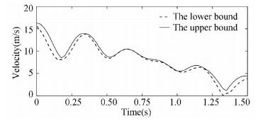
The analysis time interval is taken as t0= [0 s, 1.5 s], Δt=0.012 s, and the upper and lower bounds of speed by CIF method are shown in Fig. 5.
|
Fig.5 Lower and upper bounds of velocity |
It can be seen from Fig. 5 that the equivalent velocity shows a curve fluctuation in the time domain range. Due to the interval uncertainty of the parameters, the response value of the dynamic precision is also the interval.
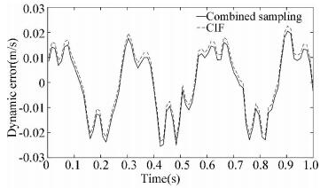
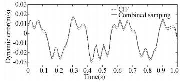
The dynamic error was calculated by Eq. (28). In order to verify the accuracy of the CP method, the combinatorial samplings were performed at each time point t. The result was compared with the CP as shown in Fig. 6 and Fig. 7.
|
Fig.6 Comparison between CIF and MCS for the upper bound |
|
Fig.7 Comparison between CIF and MCS for the lower bound |
The maximum absolute value of the dynamic accuracy in the time domain range is 0.030 89 m/s, and the corresponding time t=0.424 s, i.e., the system is most susceptible to functional failure at 0.424 s.
The threshold of maximum absolute value of dynamic error was set as Sd=0.030 m/s at 0.424 s, so the state function can be defined as:
| $ G=S_{d}-\tilde{v}_{\max }(\xi, t) $ | (30) |
where
Therefore, the non-probabilistic reliability of the dynamic accuracy can be obtained by the method described in Section 2.2. In order to verify the accuracy of the CIF, the MCS was used for comparison. The number of samples selected was 10000 and the sampling was evenly distributed. The results are shown in Table 3.
| Table 3 Result comparison of the examples |
The results show that the upper and lower bounds of the velocity response obtained by the CIF are very close to that by the MCS method, and the range of the CIF includes the solution range of the MCS. This method is more conservative in estimating reliability. The CIF only requires the sample size of 70 to provide the dynamic error range, which is much less than the 10000 sample size required by the MCS. The accuracy and high efficiency of the CIF for solving the non-probabilistic MAR of manipulators can thus be found.
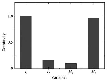
Sensitivities of interval variables are presented in Fig. 8, where the sequence of the sensitivities is l1>M2>l2>M1. The ranking shows that the uncertainty of l1 has the most significant impact on the non-probabilistic MAR. Therefore, engineering personnel can improve the non-probabilistic reliability index by reducing the uncertainty of the interval variables l1 and M2, thereby improving the structure robustness.
|
Fig.8 Sensitivity results |
5 Conclusions
An MAR analysis procedure based on CIF for manipulators involving interval parameters is proposed in this paper. In this method, the CIF was applied to evaluate the bounds for the pending function and to control the overestimation with interval methodology. The CIF method can quantify the influence of the interval uncertainty information on the dynamic response of the manipulator. Based on the interval reliability theory, the MAR of the two-link manipulator was predicted. To validate the CIF method, a MCS method was applied to calculate the MAR. As a result, the proposed method can analyze the dynamics and reliability of the manipulator with pure interval design variables. The case of two-link manipulator showed that the proposed method could solve uncertain problems with pure interval design variables efficiently. At the end of the paper, the sensitivity analysis was performed to facilitate the optimization design by using global sensitivity analysis.
| [1] |
Jr Brandhorst H W, Rodiek J A. Space solar array reliability: A study and recommendations. Acta Astronautica, 2008, 63(11-12): 1233-1238. DOI:10.1016/j.actaastro.2008.05.010 (  0) 0) |
| [2] |
Wu J, Yan S, Xie L. Reliability analysis method of a solar array by using fault tree analysis and fuzzy reasoning Petri net. Acta Astronautica, 2011, 69(11-12): 960-968. DOI:10.1016/j.actaastro.2011.07.012 (  0) 0) |
| [3] |
Huang X, Hu S, Zhang Y, et al. A method to determine kinematic accuracy reliability of gear mechanisms with truncated random variables. Mechanism and Machine Theory, 2015, 92: 200-212. DOI:10.1016/j.mechmachtheory.2015.04.017 (  0) 0) |
| [4] |
Sun D, Chen G. Kinematic accuracy analysis of planar mechanisms with clearance involving random and epistemic uncertainty. European Journal of Mechanics - A/Solids, 2016, 58: 256-261. DOI:10.1016/j.euromechsol.2016.02.007 (  0) 0) |
| [5] |
Zhou D, Zhang X F, Zhang Y M. Dynamic reliability analysis for planetary gear system in shearer mechanisms. Mechanism and Machine Theory, 2016, 105: 244-259. DOI:10.1016/j.mechmachtheory.2016.07.007 (  0) 0) |
| [6] |
Li J, Huang H, Yan S, et al. Kinematic accuracy and dynamic performance of a simple planar space deployable mechanism with joint clearance considering parameter uncertainty. Acta Astronautica, 2017, 136: 34-45. DOI:10.1016/j.actaastro.2017.02.027 (  0) 0) |
| [7] |
Wang J, Zhang J, Du X. Hybrid dimension reduction for mechanism reliability analysis with random joint clearances. Mechanism and Machine Theory, 2011, 46(10): 1396-1410. DOI:10.1016/j.mechmachtheory.2011.05.008 (  0) 0) |
| [8] |
Kakizaki T, Deck J F, Dubowsky S. Modeling the spatial dynamics of robotic manipulators with flexible links and joint clearances. Journal of Mechanical Design, 1993, 115(4): 839-847. DOI:10.1115/1.2919277 (  0) 0) |
| [9] |
Ting K-L, Zhu J, Watkins D. The effects of joint clearance on position and orientation deviation of linkages and manipulators. Mechanism and Machine Theory, 2000, 35(3): 391-401. DOI:10.1016/S0094-114X(99)00019-1 (  0) 0) |
| [10] |
Yang T, Yan S, Han Z. Nonlinear model of space manipulator joint considering time-variant stiffness and backlash. Journal of Sound and Vibration, 2015, 341: 246-259. DOI:10.1016/j.jsv.2014.12.028 (  0) 0) |
| [11] |
Lin Q, Nie H, Ren J, et al. Investigation on design and reliability analysis of a new deployable and lockable mechanism. Acta Astronautica, 2012, 73: 183-192. DOI:10.1016/j.actaastro.2011.12.004 (  0) 0) |
| [12] |
Binaud N, Cardou P, Caro S, et al. The kinematic sensitivity of robotic manipulators to joint clearances. Proceedings of the ASME Design Engineering Technical Conference, 2010, 44106: 1371-1380. DOI:10.1115/DETC2010-28635 (  0) 0) |
| [13] |
Tsai M-J, Lai T-H. Kinematic sensitivity analysis of linkage with joint clearance based on transmission quality. Mechanism and Machine Theory, 2004, 39(11): 1189-1206. DOI:10.1016/j.mechmachtheory.2004.05.009 (  0) 0) |
| [14] |
Lee S J, Gilmore B J. The determination of the probabilistic properties of velocities and accelerations in kinematic chains with uncertainty. Journal of Mechanical Design, 1991, 113(1): 84-90. DOI:10.1115/1.2912755 (  0) 0) |
| [15] |
Geng X, Wang X, Wang L, et al. Non-probabilistic time-dependent kinematic reliability assessment for function generation mechanisms with joint clearances. Mechanism and Machine Theory, 2016, 104: 202-221. DOI:10.1016/j.mechmachtheory.2016.05.013 (  0) 0) |
| [16] |
Alefeld G, Mayer G. Interval analysis: Theory and applications. Journal of Computational and Applied Mathematics, 2000, 121(1-2): 421-464. DOI:10.1016/S0377-0427(00)00342-3 (  0) 0) |
| [17] |
Viegas C, Daney D, Tavakoli M, et al. Performance analysis and design of parallel kinematic machines using interval analysis. Mechanism and Machine Theory, 2017, 115: 218-236. DOI:10.1016/j.mechmachtheory.2017.05.003 (  0) 0) |
| [18] |
Jackson K R, Nedialkov N S. Some recent advances in validated methods for IVPs for ODEs. Applied Numerical Mathematics, 2002, 42(1-3): 269-284. DOI:10.1016/S0168-9274(01)00155-6 (  0) 0) |
| [19] |
Newmark N M. A method of computation for structural dynamics. Journal of the Engineering Mechanics Division, 1959, 85(3): 67-94. (  0) 0) |
| [20] |
Qiu Z P, Wang X J. Parameter perturbation method for dynamic responses of structures with uncertain-but-bounded parameters based on interval analysis. International Journal of Solids and Structures, 2005, 42(18-19): 4958-4970. DOI:10.1016/j.ijsolstr.2005.02.023 (  0) 0) |
| [21] |
Wu J L, Luo Z, Zhang N, et al. A new interval uncertain optimization method for structures using Chebyshev surrogate models. Computers & Structures, 2015, 146: 185-196. DOI:10.1016/j.compstruc.2014.09.006 (  0) 0) |
| [22] |
Wei S, Han Q, Peng Z, et al. Dynamic analysis of parametrically excited system under uncertainties and multi-frequency excitations. Mechanical Systems and Signal Processing, 2016, 72-73: 762-784. DOI:10.1016/j.ymssp.2015.10.036 (  0) 0) |
| [23] |
Wang X, Wang L, Elishakoff I, et al. Probability and convexity concepts are not antagonistic. Acta Mechanica, 2011, 219(1-2): 45-64. DOI:10.1007/s00707-010-0440-4 (  0) 0) |
| [24] |
Wu J, Luo Z, Zhang N, et al. A new uncertain analysis method and its application in vehicle dynamics. Mechanical Systems and Signal Processing, 2015, 50-50: 659-675. DOI:10.1016/j.ymssp.2014.05.036 (  0) 0) |
| [25] |
Wu J, Zhang Y, Chen L, et al. A Chebyshev interval method for nonlinear dynamic systems under uncertainty. Applied Mathematical Modelling, 2013, 37(6): 4578-4591. DOI:10.1016/j.apm.2012.09.073 (  0) 0) |
| [26] |
Wu J, Luo Z, Zhang Y, et al. Interval uncertain method for multibody mechanical systems using Chebyshev inclusion functions. International Journal for Numerical Methods in Engineering, 2013, 95(7): 608-630. DOI:10.1002/nme.4525 (  0) 0) |
| [27] |
Shen Z, Li P, Liu C, et al. A finite element beam model including cross-section distortion in the absolute nodal coordinate formulation. Nonlinear Dynamics, 2014, 77(3): 1019-1033. DOI:10.1007/s11071_014_1360_y (  0) 0) |
| [28] |
Wang Z, Tian Q, Hu H. Dynamics of flexible multibody systems with hybrid uncertain parameters. Mechanism and Machine Theory, 2018, 121: 128-147. DOI:10.1016/j.mechmachtheory.2017.09.024 (  0) 0) |
 2019, Vol. 26


