1 Introduction

On-orbit spacecraft face with failures and faults due to severe space environment^[1]. On average dozens of spacecraft are destroyed every year, and on-orbit servicing can be carried out to these spacecraft such as International Space Station (ISS) and Hubble Telescope. Spacecraft on-orbit servicing (OOS) including spacecraft maintenance, on-orbit assembly, refueling, and de-orbiting can reduce the cost of space missions, improve the performance of spacecraft, and extend its life span^[1]. Therefore, this is of great interest for many countries^[2]. For example, the Orbital Express program^[3] was an OOS demonstration program to verify the technical feasibility of on-board robots maintaining on-orbit satellites and demonstrate on-orbit interactive docking. ROKVISS was part of German space robot research project to verify various teleoperation control modes of space robots and accumulate experience for future design and operation of space robots for on-orbit service^[4].

The position and attitude of the target relative to the servicing spacecraft is vitally important for OOS missions, which can be divided into remote guiding stage, approaching stage, final translation, and contact stage. Several measure methods can be used for different stages, such as GPS for the remote guiding stage, laser radar for approaching stage, and visual navigation for the final stage. This paper focuses on the final approaching stage as mentioned above, and a low-cost monocular vision system is implemented to supply the relative translation and rotation. It is a tough problem for the relative pose estimation of the final approaching stage to a non-cooperative spacecraft, as no artificial markers on the target spacecraft are available.

Non-cooperative spacecraft cannot provide cooperative markers for auxiliary measurement, and it has no information exchange with the servicing spacecraft. Even its state is uncontrollable^[5-6]. Therefore, the relative navigation of non-cooperative spacecraft relies entirely on the external observation to autonomously achieve real-time high-precision measurement of the relative motion without cooperative identity and inter-spacecraft data exchange. As a key technology of on-orbit servicing, relative states measuring for the non-cooperative spacecraft has become a research hotspot and received wide attention from various countries in recent years.

The spacecraft motion can be divided into orbital and attitude motion. Traditional dynamic model usually describes the two motions separately, ignoring the coupling effects of orbit and attitude.To deal with this problem, Refs. [7-9] considered the coupling effect of orbit and attitude to establish a six-degree-of-freedom spacecraft motion dynamics model, but used different mathematical tools to describe the orbit and attitude parameters.It is difficult to achieve a truly integrated coupled dynamics modeling. Dual quaternion can represent the general motion of a rigid body simply and effectively. Therefore, it was used to model the spacecraft coupled dynamics.The dual quaternion can not only represent the attitude, but also the position of the rigid body.Compared with other representation methods of rigid bodies in three-dimensional space, dual quaternion method has a simple concept and clear geometric meaning, and has no singularity^[10].

Kalman filter (KF) is a recursive linear minimum variance estimation. It not only strongly depends on the system model, but also loses the ability to track the abrupt state when the system reaches the stationary state. Therefore, the tracking ability of this method is limited with poor robustness. Extended Kalman filter (EKF) is the most widely used state estimation method at present.Nevertheless, the established system model has many uncertainties when the target is non-cooperative. The stability of extended Kalman filter is poor. To handle this problem, Ref. [11] adjusted the extended filter gain matrix and the state error variance matrix to force the filter to meet the principle of orthogonality, so that the estimated state of the filter can keep track of the system's actual state. The filter has strong tracking ability because it reduces the impact of previous data on the current estimation and makes more use of current measurement data. Thus, it is called strong tracking filter (STF).

Compared with EKF, STF has improved convergence and dynamic performance as well. Its advantages include 1) strong ability to track mutation states, 2) strong robustness about model uncertainty, 3) lower sensitivity to noise and initial statistical properties, and 4) moderate computational complexity^[12]. However, the tracking function of the STF is still not ideal when the state transition is small, because the fading factor is too small when the state is abrupt. An improved strong tracking filter is proposed in Ref. [13]. The probability of misjudging filter divergence is reduced by properly increasing the threshold of judging filter divergence. Different weakening factors can be determined according to different dimensional quantitative equation, thus avoiding the defect of adding weakening factors based on experience. Ref. [14] proposes a strong tracking finite-difference Kalman filter (STFDEKF). The strong tracking filter factor is introduced to adjust the state pre-covariance matrix of the filter so that the filtering precision is improved.

Based on dual quaternion, an integrated spacecraft relative dynamics model is established. Aiming at the problem of selecting weakening factor and calculating multi-suboptimal fading matrix in STF, a fuzzy strong tracking filter with fuzzy adaptive characteristics is proposed. The method uses a fuzzy logic adaptive controller (FLAC) to dynamically modify the weakening factor, thereby adaptively adjusting the multiple sub-optimal fading matrices online, and further improving the filter tracking accuracy. The effectiveness of the method is verified by numerical simulations.

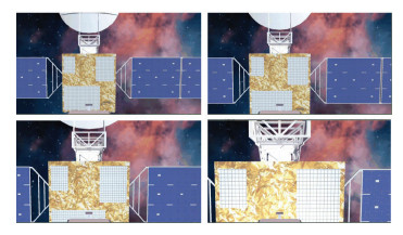
2 Scenario Analysis

The relative distance is quite short in the final approaching stage, so the measurement accuracy, which directly affects the success of on-orbit service tasks, is required to be extremely high. With the two spacecraft getting closer and closer, the camera FOV of the servicing spacecraft becomes smaller and smaller, thus fewer features can be observed. This makes it more difficult to calculate the relative position and attitude. From the perspective of servicing spacecraft, Fig. 1 presents four snaps of the target spacecraft from different distance during the approaching stage, showing that some features are missing.

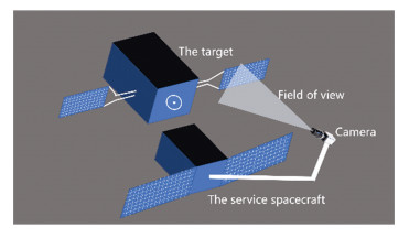
The measurement strategy in Ref. [15] is used to overcome the above issues. As shown in Fig. 2, a "selfie stick" structure and a self-calibration strategy are implemented, ensuring that part of the contour features can be observed precisely before the two spacecraft contact and part of the target spacecraft structure is within the field of view of the visual camera. The installation structure can effectively increase the distance between the camera and the target. Even if the relative distance between serving spacecraft and target is almost zero, the observation distance between the camera and the target is still about 2 m.

3 Mathematic Modeling 3.1 Coordinate Frames

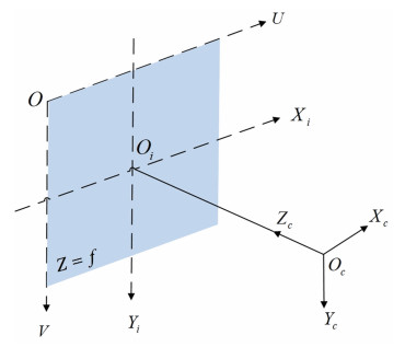
Five coordinate frames (as shown in Fig. 3) are defined as follows:

1) Servicing Spacecraft Coordinate Frame O_fX_fY_fZ_f: The origin is located at the center of mass of the servicing spacecraft, and the three axes are parallel to the corresponding inertia axes.

2) Target Coordinate Frame O_lX_lY_lZ_l: The origin is located at the center of mass of the target with its three axes parallel to the inertia axes of the target.

3) Pixel Coordinate System OUV: The origin is in the upper left corner of the image, and the horizontal axis OU and the vertical axis OV are parallel to the image plane coordinate system, respectively. The abscissa U and the ordinate V are the number of columns and rows in their image arrays, respectively.

4) Image Plane Coordinate Frame O_iX_iY_i: The origin of this frame at the intersection of the image plane and the optical axis, the X_i and Y_i axes are parallel to the horizontal and vertical directions.

5) Camera Coordinate Frame O_cX_cY_cZ_c: The origin is at the center of the camera. X_c and Y_c axes are parallel to the X_i and Y_i axes of the Image Plane Coordinate Frame, Z_c axis is vertical to the image plane.

3.2 Dual Quaternion

The concept of dual number is defined as:

$ \hat a = a + \varepsilon a' $

(1)

where a, a′∈ R, and a is the real part while a′ is the dual part of the dual number. ε is a new element with the property ε²=0.

Dual quaternion can be regarded as a quaternion, whose element is dual number, or can be written as a dual number whose element is quaternion, such as

$ \mathit{\boldsymbol{\hat q}} = \left[ {\mathit{\boldsymbol{\hat \eta }},\mathit{\boldsymbol{\hat \xi }}} \right] = \mathit{\boldsymbol{q}} + \varepsilon \mathit{\boldsymbol{p}} $

(2)

where $\hat{\boldsymbol{\eta}}$ is dual number, $\hat{\boldsymbol{\xi}} $ is dual vector, and q, p are all quaternion.

The basic operation rules for dual quaternion are as follows:

$ {{\mathit{\boldsymbol{\hat q}}}_1} + {{\mathit{\boldsymbol{\hat q}}}_2} = \left[ {{{\mathit{\boldsymbol{\hat \eta }}}_1} + {{\mathit{\boldsymbol{\hat \eta }}}_2},{{\mathit{\boldsymbol{\hat \xi }}}_1} + {{\mathit{\boldsymbol{\hat \xi }}}_2}} \right] $

(3a)

$ \lambda \mathit{\boldsymbol{\hat q}} = \left[ {\lambda \mathit{\boldsymbol{\hat \eta }},\lambda \mathit{\boldsymbol{\hat \xi }}} \right] $

(3b)

$ {{\mathit{\boldsymbol{\hat q}}}_1} \cdot {{\mathit{\boldsymbol{\hat q}}}_2} = \left[ {{{\mathit{\boldsymbol{\hat \eta }}}_1}{{\mathit{\boldsymbol{\hat \eta }}}_2} - {{\mathit{\boldsymbol{\hat \xi }}}_1} \cdot {{\mathit{\boldsymbol{\hat \xi }}}_2},{{\mathit{\boldsymbol{\hat \eta }}}_1}{{\mathit{\boldsymbol{\hat \xi }}}_2} + {{\mathit{\boldsymbol{\hat \eta }}}_2}{{\mathit{\boldsymbol{\hat \xi }}}_1} + {{\mathit{\boldsymbol{\hat \xi }}}_1} \times {{\mathit{\boldsymbol{\hat \xi }}}_2}} \right] $

(3c)

$ {{\mathit{\boldsymbol{\hat q}}}^*} = \left[ {\mathit{\boldsymbol{\hat \eta }}, - \mathit{\boldsymbol{\hat \xi }}} \right] $

(3d)

$ {\left\| {\mathit{\boldsymbol{\hat q}}} \right\|^{\rm{2}}} = \mathit{\boldsymbol{\hat q}} \cdot {{\mathit{\boldsymbol{\hat q}}}^*} $

(3e)

$ {{\mathit{\boldsymbol{\hat q}}}^{ - 1}} = {\left\| {\mathit{\boldsymbol{\hat q}}} \right\|^{ - 1}} \cdot {{\mathit{\boldsymbol{\hat q}}}^*} $

(3f)

where λ is a constant, $\hat{\boldsymbol{q}}$^* is the conjugate of $\hat{\boldsymbol{q}}$, "·" represents multiplication of the dual quaternion, and ‖·‖ is the modulus of dual quaternion.

3.3 Relative Orbit and Attitude Dynamics

The dual quaternion were used to realize the transformation from the target coordinate frame to the servicing spacecraft coordinate frame. The attitude of the target relative to the servicing spacecraft is assumed to be q_fl. The position of O_f relative to O_l described in the servicing spacecraft coordinate frame is set as r_fl^f. Then dual quaternion can be written as

$ {{\mathit{\boldsymbol{\hat q}}}_{fl}} = \mathit{\boldsymbol{\hat q}}_1^* \cdot {{\mathit{\boldsymbol{\hat q}}}_f} = {\mathit{\boldsymbol{q}}_{f l}} + \varepsilon \left( {\frac{1}{2}{\mathit{\boldsymbol{q}}_{fl}} \cdot \mathit{\boldsymbol{r}}_{fl}^f} \right) $

(4)

where the dual quaternion of the target and the servicing spacecraft in the inertial coordinate system is expressed as $\hat{\boldsymbol{q}}_l$ and $\hat{\boldsymbol{q}}_f$. q_fl is the attitude quaternion of the servicing spacecraft relative to the target. r_fl^f=r_f^f-r_l^f is the servicing spacecraft's position vector relative to the center of mass of the target in O_fX_fY_fZ_f.

Then the relative dynamics equation is

$ {{\mathit{\boldsymbol{\dot {\hat q}}}}_{fl}} = \frac{1}{2}{{\mathit{\boldsymbol{\hat q}}}_{fl}} \cdot \mathit{\boldsymbol{\hat \omega }}_{fl}^f $

(5)

where $\hat{\boldsymbol{\omega}}_{f l}^{f}=\boldsymbol{\omega}_{f l}^{f}+\varepsilon\left(\boldsymbol{r}_{f l}^{f}+\boldsymbol{\omega}_{f l}^{f} \times \boldsymbol{r}_{f l}^{f}\right) $ is the relative velocity curl in O_fX_fY_fZ_f. ω_fl^f is relative angular velocity in O_fX_fY_fZ_f. The dual inertia matrix of a rigid body spacecraft is expressed as

$ \hat M = \frac{{\rm{d}}}{{{\rm{d}}\mathit{\boldsymbol{\varepsilon }}}}\mathit{\boldsymbol{mI}} + \varepsilon J $

(6)

where m and J are the mass and inertia matrix of the spacecraft, I is identity matrix. Then the relative dynamics equation can also be described by

$ \mathit{\boldsymbol{\hat \omega }}_{fl}^f = \mathit{\boldsymbol{\omega }}_{fl}^f - \mathit{\boldsymbol{\hat q}}_{fl}^* \cdot \mathit{\boldsymbol{\hat \omega }}_l^l \cdot {\mathit{\boldsymbol{q}}_{fl}} $

(7)

Derivation on both sides of the above equation can obtain

$ \begin{array}{l} \mathit{\boldsymbol{\dot {\hat \omega} }}_{fl}^f = \mathit{\boldsymbol{\dot {\hat \omega} }}_f^f - \mathit{\boldsymbol{\dot {\hat q}}}_{fl}^* \cdot \mathit{\boldsymbol{\hat \omega }}_l^l \cdot {{\mathit{\boldsymbol{\hat q}}}_{fl}} - \mathit{\boldsymbol{\hat q}}_{fl}^* \cdot \mathit{\boldsymbol{\dot {\hat \omega} }}_l^l \cdot {{\mathit{\boldsymbol{\hat q}}}_{fl}} - \\ \mathit{\boldsymbol{\hat q}}_{fl}^* \cdot \mathit{\boldsymbol{\hat \omega }}_l^l \cdot {{\mathit{\boldsymbol{\dot {\hat q}}}}_{fl}} = - \mathit{\boldsymbol{\hat M}}_f^{ - 1}\left( {\mathit{\boldsymbol{\hat \omega }}_f^f \times {{\mathit{\boldsymbol{\hat M}}}_f}\mathit{\boldsymbol{\hat \omega }}_f^f - \mathit{\boldsymbol{\hat F}}_f^f} \right) - \\ \mathit{\boldsymbol{\hat q}}_{fl}^* \cdot \mathit{\boldsymbol{\dot {\hat \omega} }}_l^l \cdot {{\mathit{\boldsymbol{\hat q}}}_{fl}} - \mathit{\boldsymbol{\hat q}}_{fl}^* \cdot \mathit{\boldsymbol{\hat \omega }}_l^l \cdot \frac{1}{2}{{\mathit{\boldsymbol{\hat q}}}_{fl}} \cdot \mathit{\boldsymbol{\hat \omega }}_{fl}^l + \\ \frac{1}{2}\mathit{\boldsymbol{\hat \omega }}_{fl}^l \cdot \mathit{\boldsymbol{\hat q}}_{fl}^ * \cdot \mathit{\boldsymbol{\hat \omega }}_l^l \cdot {{\mathit{\boldsymbol{\hat q}}}_{fl}} = \\ - \mathit{\boldsymbol{\hat M}}_f^{ - 1}\left( {\mathit{\boldsymbol{\hat \omega }}_f^f \times {{\mathit{\boldsymbol{\hat M}}}_f}\mathit{\boldsymbol{\hat \omega }}_f^f - \mathit{\boldsymbol{\hat F}}_f^f} \right) - \\ \mathit{\boldsymbol{\hat q}}_{fl}^* \cdot \mathit{\boldsymbol{\dot {\hat \omega} }}_l^l \cdot {{\mathit{\boldsymbol{\hat q}}}_{fl}} + \mathit{\boldsymbol{\hat \omega }}_{fl}^f \times \left( {\mathit{\boldsymbol{\hat q}}_{fl}^* \cdot \mathit{\boldsymbol{\hat \omega }}_l^l \cdot {{\mathit{\boldsymbol{\hat q}}}_{fl}}} \right) \end{array} $

(8)

where, $\hat{\boldsymbol{F}}_{f}^{f}$ is the dual force curl on the servicing spacecraft centroid, $\hat{\boldsymbol{M}}_{f}$ is the dual inertia matrix for the servicing spacecraft, and $\hat{\boldsymbol{M}}_{f}^{-1}$ is the inverse of the dual inertia matrix. $ \hat{\boldsymbol{\omega}}_{f}^{f}$ is the velocity curl of the servicing spacecraft in O_fX_fY_fZ_f, and $\hat{\boldsymbol{\omega}}_{l}^{l} $ is the velocity curl of the target in O_lX_lY_lZ_l.

The model based on dual quaternion is different from modeling methods. It does not simply overlap the two independent models of position and attitude, but the two parts should be coupled. The final dynamic model can express the interaction relationship.

4 Measurement Equation

Spacecraft has obvious external features, such as corners of main body, edges of the solar sail bracket, and central docking ring. Extracting single feature may not only result in less information, but also reduce the accuracy of estimation results. These problems can be solved by extracting multiple features and implementing data fusion. It is necessary to consider how to represent different measurements of points, lines, and circles with one model. Therefore, the measurement model in Ref. [16] is cited.

4.1 Point

The dual quaternion of any point P in the target coordinate frame is expressed as $ \hat{\boldsymbol{D}}^{l P}=1-\varepsilon \boldsymbol{d}^{l P}$, where the dual part d^lP is the component of P in the coordinate frame. Then the point in the servicing spacecraft coordinate frame is written as

$ {{\mathit{\boldsymbol{\hat D}}}^{fP}} = \mathit{\boldsymbol{\hat q}}_{fl}^ * \cdot {{\mathit{\boldsymbol{\hat D}}}^{lP}} \cdot {{\mathit{\boldsymbol{\hat q}}}_{fl}} $

(9)

where $\hat{\boldsymbol{q}}_{fl}$ is the dual quaternion from O_fX_fY_fZ_f to O_lX_lY_lZ_l. $ \hat{\boldsymbol{q}}_{fl}^{*}=\boldsymbol{q}_{fl}^{*}-\boldsymbol{p}_{fl}^{*}$ is the corresponding conjugate dual quaternion. $ \hat{\boldsymbol{q}}_{c f}$ is defined as the dual quaternion from O_fX_fY_fZ_f to O_cX_cY_cZ_c. Then point P can be expressed in the camera coordinate frame as

$ {{\mathit{\boldsymbol{\hat D}}}^{cP}} = \mathit{\boldsymbol{\hat q}}_{cf}^* \cdot {{\mathit{\boldsymbol{\hat D}}}^{fP}} \cdot {{\mathit{\boldsymbol{\hat q}}}_{cf}} $

(10)

where $ \hat{\boldsymbol{D}}_{c P}=1-\varepsilon \boldsymbol{d}^{c P}, \boldsymbol{d}^{c P}=\left[\begin{array}{ccc} {d_{x}^{c P}} & {d_{y}^{c P}} & {d_{z}^{c P}} \end{array}\right]^{T}$. If f is the focal length of the camera, the coordinates of point P on the image plane d^iP=[d_x^iP d_y^iP]^T is

$ \mathit{\boldsymbol{d}}_x^{iP} = f\frac{{\mathit{\boldsymbol{d}}_x^{cP}}}{{\mathit{\boldsymbol{d}}_z^{cP}}},\mathit{\boldsymbol{d}}_y^{iP} = f\frac{{\mathit{\boldsymbol{d}}_y^{cP}}}{{\mathit{\boldsymbol{d}}_z^{cP}}} $

(11)

4.2 Line

Any line in the target spacecraft is defined as $ \hat{\boldsymbol{L}}=\boldsymbol{l}^{l}+\varepsilon \boldsymbol{m}^{l} $, where l^l is the unit direction vector of the line, and m^l is the moment from the origin to the line, then the line in the camera coordinate frame is

$ {{\mathit{\boldsymbol{\hat L}}}^c} = {\mathit{\boldsymbol{l}}^c} + \varepsilon {\mathit{\boldsymbol{m}}^c} = \mathit{\boldsymbol{\hat q}}_{cf}^* \cdot \mathit{\boldsymbol{\hat q}}_{fl}^* \cdot {{\mathit{\boldsymbol{\hat L}}}^l} \cdot {{\mathit{\boldsymbol{\hat q}}}_{fl}} \cdot {{\mathit{\boldsymbol{\hat q}}}_{cf}} $

(12)

The conjugate dual quaternion of the line is $\hat{\boldsymbol{q}}_{f l}^{*}= \boldsymbol{q}_{f l}^{*}+{\varepsilon} \boldsymbol{p}_{fl}^{*}$. The projection of the feature line in the target on the camera image plane is shown in Fig. 4.

The normal vector of the plane formed by the feature line and the origin of the camera coordinate system is m^c=[m_c^x m_c^y m_c^z]^T, and image plane equation is z=-f. The intersection of the image plane and the plane formed by the feature line and the camera's origin is the projection of the feature line in the image plane, i.e.

$ m_x^cx + m_y^cy + m_z^cf = 0 $

(13)

It can be obtained that the pedal coordinate from the origin of the image plane coordinate system to the projection line is

$ {x_{iL}} = f\frac{{m_x^cm_z^c}}{{{{\left( {m_x^c} \right)}^2} + {{\left( {m_y^c} \right)}^2}}} $

(14a)

$ {y_{iL}} = f\frac{{m_y^cm_z^c}}{{{{\left( {m_x^c} \right)}^2} + {{\left( {m_y^c} \right)}^2}}} $

(14b)

4.3 Circle

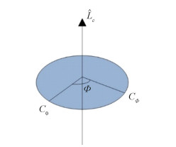
Any circle C on the target spacecraft can be defined by the rotation characteristics of the circle C_ir. The start point of the circle is C₀, the axis of rotation is $ \hat{\boldsymbol{L}}_{c}$, and the feature circle is obtained by rotating the start point along the rotation axis. The feature circle can be determined by three end points C_Φ, which are obtained by rotating the start point with three different angles Φ, as shown in Fig. 5.

Define the start point of the feature circle as $\boldsymbol{\hat{C}}_{0}^{l}= 1-\varepsilon \boldsymbol{d}_{c 0}$, the dual quaternion of the rotational motion is described as

$ {{\mathit{\boldsymbol{\hat q}}}_\mathit{\Phi }} = \left[ {\cos \frac{\mathit{\Phi }}{2},{{\mathit{\boldsymbol{\hat L}}}_c}\sin \frac{\mathit{\Phi }}{2}} \right] $

(15)

In the frame O_lX_lY_lZ_l, $ \hat{\boldsymbol{C}}_{\varPhi}^{l}$ is expressed as

$ \mathit{\boldsymbol{\hat C}}_\mathit{\Phi }^l = 1 - \varepsilon \mathit{\boldsymbol{d}}_\mathit{\Phi }^l = {{\mathit{\boldsymbol{\hat q}}}_\mathit{\Phi }} \cdot \mathit{\boldsymbol{\hat C}}_\mathit{\Phi }^l \cdot \mathit{\boldsymbol{q}}_\mathit{\Phi }^ * $

(16)

The above equation represents the transformation of different points in the same coordinate frame, which is opposite to the conversion of the same points in different coordinate frames. The conjugate form of the dual quaternion is consistent with the conjugate form of feature point transformation. The end point is expressed in the Camera Coordinate Frame as

$ \mathit{\boldsymbol{\hat C}}_\mathit{\Phi }^c = 1 - \varepsilon \mathit{\boldsymbol{d}}_\mathit{\Phi }^c = \mathit{\boldsymbol{\hat q}}_{cf}^* \cdot \mathit{\boldsymbol{\hat q}}_{fl}^* \cdot \mathit{\boldsymbol{\hat C}}_\mathit{\Phi }^l \cdot {{\mathit{\boldsymbol{\hat q}}}_{fl}} \cdot {{\mathit{\boldsymbol{\hat q}}}_{cf}} $

(17)

where $\boldsymbol{d}_{\varPhi}^{c}=\left[\begin{array}{lll} {d_{\varPhi{x}}^{c}} & {d_{\varPhi{y}}^{c}} & {d_{\varPhi{z}}^{c}} \end{array}\right]^{{\rm T}} $, and the projection coordinates of the end point in the image plane are

$ d_{\mathit{\Phi }x}^i = f\frac{{d_{\mathit{\Phi }x}^c}}{{d_{\mathit{\Phi }z}^c}} $

(18a)

$ d_{\mathit{\Phi }y}^i = f\frac{{d_{\mathit{\Phi }y}^c}}{{d_{\mathit{\Phi }z}^c}} $

(18b)

5 Relative Pose Estimation Method

EKF is usually used to estimate the states of the system with poor tracking performance. STF has been improved on the basis of EKF. The tracking speed is relatively improved, but the fixed weakening factor reduces the accuracy of the algorithm. Based on Refs. [12-14], an improved strong tracking Kalman filter with fuzzy adaptive characteristics is proposed considering both positive and negative observation residuals.

5.1 Strong Tracking Filter

Consider a linear constant system.

$ {\mathit{\boldsymbol{x}}_k} = {\mathit{\boldsymbol{F}}_{k - 1}}{\mathit{\boldsymbol{x}}_{k - 1}} + {\mathit{\boldsymbol{W}}_{k - 1}} $

(19a)

$ {\mathit{\boldsymbol{z}}_k} = {\mathit{\boldsymbol{H}}_k}{\mathit{\boldsymbol{x}}_k} + {\mathit{\boldsymbol{V}}_k} $

(19b)

where k≥0 and k is an integer. x_k is a state variable, F_k-1 is the state transition matrix, z_k is the observed variable, and H_k is the observed matrix. W_k-1 and V_k are respectively process noise and measurement noise that can be regarded as Gaussian white noise. Q_k and R_k are the process noise variance matrix and the measurement noise variance matrix, respectively.

The expression operation of the STF is as follows:

$ {\mathit{\boldsymbol{x}}_k} = {\mathit{\boldsymbol{x}}_{k\left| {k - 1} \right.}} + {\mathit{\boldsymbol{K}}_k}{\mathit{\boldsymbol{\gamma }}_k} $

(20a)

$ {\mathit{\boldsymbol{P}}_k} = \left[ {\mathit{\boldsymbol{I}} - {\mathit{\boldsymbol{K}}_k}{\mathit{\boldsymbol{H}}_{k\left| {k - 1} \right.}}} \right]{\mathit{\boldsymbol{P}}_{k\left| {k - 1} \right.}} $

(20b)

where

$ {\mathit{\boldsymbol{x}}_{k\left| {k - 1} \right.}} = f\left( {{\mathit{\boldsymbol{x}}_{k - 1}},{\mathit{\boldsymbol{u}}_{k - 1}}} \right) $

$ {\mathit{\boldsymbol{P}}_{k\left| {k - 1} \right.}} = {\mathit{\boldsymbol{\lambda }}_k}\left( {{\mathit{\boldsymbol{F}}_{k - 1}}{\mathit{\boldsymbol{P}}_{k - 1}}\mathit{\boldsymbol{F}}_{k - 1}^{\rm{T}} + {\mathit{\boldsymbol{Q}}_{k - 1}}} \right) $

$ {\mathit{\boldsymbol{K}}_k} = {\mathit{\boldsymbol{P}}_{k\left| {k - 1} \right.}}\mathit{\boldsymbol{H}}_{k\left| {k - 1} \right.}^{\rm{T}}{\left( {{\mathit{\boldsymbol{H}}_{k\left| {k - 1} \right.}}{\mathit{\boldsymbol{P}}_{k\left| {k - 1} \right.}} + {\mathit{\boldsymbol{R}}_k}} \right)^{ - 1}} $

$ {\mathit{\boldsymbol{H}}_{k\left| {k - 1} \right.}} = {\left. {\frac{{\partial \mathit{\boldsymbol{h}}}}{{\partial {\mathit{\boldsymbol{x}}^{\rm{T}}}}}} \right|_{x = {x_{k\left| {k - 1} \right.}}}} $

The fading factor λ_k can be obtained by

$ {\mathit{\boldsymbol{\lambda }}_k} = \max \left( {1,\frac{{{\rm Tr}\left( {{\mathit{\boldsymbol{N}}_k}} \right)}}{{{\rm Tr}\left( {{\mathit{\boldsymbol{M}}_k}} \right)}}} \right) $

(21)

where

$ {\mathit{\boldsymbol{N}}_k} = {\mathit{\boldsymbol{C}}_{0,k}} - \beta {\mathit{\boldsymbol{R}}_k} $

$ {\mathit{\boldsymbol{M}}_k} = {\mathit{\boldsymbol{H}}_{k\left| {k - 1} \right.}}\left[ {{\mathit{\boldsymbol{F}}_{k - 1}}{\mathit{\boldsymbol{P}}_{k - 1}}\mathit{\boldsymbol{F}}_{k - 1}^{\rm{T}} + {\mathit{\boldsymbol{Q}}_{k - 1}}} \right]\mathit{\boldsymbol{H}}_{k\left| {k - 1} \right.}^{\rm{T}} $

$ {\mathit{\boldsymbol{C}}_{0,k}} = \left\{ \begin{array}{l} {\mathit{\boldsymbol{\gamma }}_1}\mathit{\boldsymbol{\gamma }}_1^{\rm{T}},\;\;\;\;\;\;\;\;\;\;\;\;\;\;k = 0\\ \frac{{\rho {\mathit{\boldsymbol{C}}_{0,k - 1}} + {\mathit{\boldsymbol{\gamma }}_k}\mathit{\boldsymbol{\gamma }}_k^{\rm{T}}}}{{1 + \rho }},k \ge 1 \end{array} \right. $

Among them, 0.95≤ρ≤0.995 is a forgetting factor. It can be seen from the above formula that STF is essentially a Kalman filter which has multiple time-varying fading factors, and the role of which is extremely important. When the system state changes abruptly, an increase in the estimated error γ_k will cause an increase in the error variance matrix C_{0, k} and the filter tracking capability, thereby improving the dynamic performance of the filter.

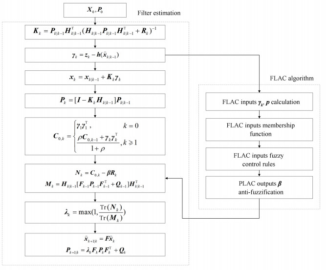
5.2 Fuzzy Adaptive Strong Tracking Filter

The above analysis shows that the existing STF uses a fixed weakening factor, which needs to be selected by experience or numerical simulations. However, it is impossible to establish accurate mathematical models. To solve this problem, a fuzzy adaptive strong tracking filter (FASTF) is proposed by combining fuzzy logic adaptive controller with STF. The flow chart of the algorithm is shown in Fig. 6.

As is shown that the state estimation algorithm in FASTF is the same as STF, but the difference is that the "online" adaptive adjustment of the weakening factor β and the multiple suboptimal fading factor λ_k is realized by FLAC. It is an intelligent control method, and it mimics human fuzzy reasoning and decision-making process^[17-18]. The method first compiles the operator or expert experience into fuzzy rules, then blurs the real-time signal, and uses the fuzzified signal as the input of the fuzzy rule. The input of FLAC is the statistical feature quantity of the system (residual and variance). According to the fuzzy inference rule, the nonlinear adjustment of β is realized, thereby improving the filter estimation accuracy. The specific design of FLAC is as below:

1) Fuzzy set of input and output.

The inputs of FLAC are the residual γ_k and variance p at the current moment:

$ {\mathit{\boldsymbol{\gamma }}_k} = {\mathit{\boldsymbol{z}}_k} - \mathit{\boldsymbol{h}}\left( {{{\mathit{\boldsymbol{\mathord{\buildrel{\lower3pt\hbox{$\scriptscriptstyle\frown$}} \over x} }}}_{k\left| {k - 1} \right.}}} \right) $

$ \mathit{\boldsymbol{p}} = {\mathit{\boldsymbol{\gamma }}_k}\mathit{\boldsymbol{\gamma }}_k^{\rm{T}} $

The state variable of the system x is

$ \mathit{\boldsymbol{x}} = {\left[ {\mathit{\boldsymbol{q}}_{fl,P}^{\rm{T}},\mathit{\boldsymbol{\omega }}_{fl,P}^{fP{\rm{T}}},{\mathit{\boldsymbol{ \boldsymbol{\varPhi} }}^{\rm{T}}}} \right]^{\rm{T}}} $

where $\hat{\boldsymbol{q}}_{fl, P} $ is the dual quaternion of relative motion, $\hat{\boldsymbol{\omega}}_{fl, P}^{fP} $ is the relative velocity curl, and Φ=[Φ₁, Φ₂, Φ₃]^T is the unknown parameter related to the observation of a certain circle. The geometric feature on the spacecraft is observed, which includes the feature point, feature line, and the feature circle. The fuzzy sets of residual γ_k, variance p, weakening factor β, and their domains are defined in Table 1.

2) Input and output membership functions.

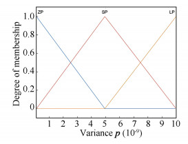
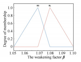
After the fuzzy sets and the domains of the residual γ_k, variance p and weakening factor β are determined. It is necessary to determine the membership function of fuzzy variables, that is, to assign values to fuzzy variables, and to determine the membership degree of elements in the domain to fuzzy variables.

The inputs γ_k and p of FLAC are fuzzified according to the membership functions shown in Figs. 7-8. The membership function of the output β of FLAC is shown in Fig. 9.

3) Fuzzy control rules.

The fuzzy control rule can be described in Table 2. There are 15 rules in the table. The relationship between each fuzzy statement is "or", and the control rule determined by the first statement can calculate β₁. Similarly, β₂, β₃, ..., β₁₅ can be obtained from the remaining statements, and the weakening factor is the fuzzy set β, which can be expressed as

$ \mathit{\boldsymbol{\beta }} = \left\{ {{\beta _1},{\beta _2}, \ldots ,{\beta _{15}}} \right\} $

It should be noted that the weakening factor β can be expressed as a diagonal matrix with the same dimension as R, and the diagonal elements are the weakening factor components corresponding to the observed components. The weakening factor components are adaptively adjusted by FLAC designed above.

4) Anti-fuzzification.

The result obtained by fuzzy inference is a fuzzy set. However, there must be a certain value to control the object in actual fuzzy control. The process of transforming fuzzy inference results into exact values is called anti-fuzzification.

In order to obtain an accurate control amount, the fuzzy method is required to express the calculation result of the output membership function well. The centroid method is to use the center of gravity of the area surrounded by the membership function curve and the abscissa as the final output value of the fuzzy inference. For the discrete domain with m output quantization series, there is

$ {v_o} = \frac{{\sum\limits_{k = 1}^m {{v_h}} {\mu _v}\left( {{v_k}} \right)}}{{\sum\limits_{k = 1}^m {{\mu _v}} \left( {{v_k}} \right)}} $

The center of gravity method has smooth output inference control.The output changes even if it corresponds to a small change in the input signal.

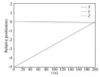
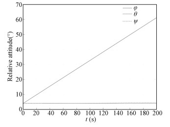
6 Numerical Simulation and Analysis

Assuming that the target spacecraft is in GEO orbit, the relative translation between the servicing and the target spacecraft can be regarded as a line approaching motion because the relative distance and maneuvering time are rather short compared with the orbital period of the target. The servicing spacecraft is approaching the target with a velocity of about 0.025 m/s, and the target rotates around the x axis with an angular velocity of about 0.005 rad/s. The initial reference relative states are q_fl= [0.998 2, 0.033 6, 0.033 6, 0.033 6]^T and γ_fl^f=[0, -5, 0, 0]^T m, ω_fl^f=[0, 0.005, 0, 0]^T rad/s, and ν_fl^f=[0, 0.025, 0, 0]^T m/s. The corresponding relative position and attitude are presented in Figs. 10-11.

The mass and moment of inertia of the servicing spacecraft are

$ {m_f} = 100~{\rm{kg}},{\mathit{\boldsymbol{J}}_f} = {\rm diag}\left( {4,4.2,3.8} \right){\rm{kg}} \cdot {{\rm{m}}^2} $

The estimated initial relative states are set as

$ {{\mathit{\boldsymbol{\bar q}}}_{fl}} = {\left[ {0.9995,0.0171,0.0178,0.0171} \right]^{\rm{T}}} $

$ \mathit{\boldsymbol{\bar r}}_{fl}^f = {\left[ {0, - 5.3,0.1,0.1} \right]^{\rm{T}}}{\rm{m}} $

The initial position of the camera is

$ {\mathit{\boldsymbol{q}}_{cf}} = {\left[ {1,0,0,0} \right]^{\rm{T}}},\mathit{\boldsymbol{r}}_{cf}^c = {\left[ {0,1,1, - 1.5} \right]^{\rm{T}}}{\rm{m}} $

Considering the robustness of the STF, the following uncertainties are considered and introduced into the model:

$ {m_f} = \left( {1 + \delta } \right){m_f},{\mathit{\boldsymbol{J}}_f} = \left( {1 + \delta } \right){\mathit{\boldsymbol{J}}_f},{\mathit{\boldsymbol{\omega }}_l} = \left( {1 + \delta } \right){\mathit{\boldsymbol{\omega }}_l} $

where δ=0.1.

For the relative distance from 5 m to 3 m, points, line, and circle on the target spacecraft can be observed. The coordinates of the four feature points are

$ \mathit{\boldsymbol{d}}_1^l = {\left[ {0,1,0.4,0.5} \right]^{\rm{T}}},\mathit{\boldsymbol{d}}_2^l = {\left[ {0,1, - 0.4,0.5} \right]^{\rm{T}}} $

$ \mathit{\boldsymbol{d}}_3^l = {\left[ {0,0.7,0,0.5} \right]^{\rm{T}}},\mathit{\boldsymbol{d}}_4^l = {\left[ {0,0.5,0.5,0} \right]^{\rm{T}}} $

The feature line is described as $ \hat{\boldsymbol{L}}_{1}^{l}=[0, 0, 1, 0]^{\mathrm{T}}+$ε[0, 0, 0, 0.5]^T. The axis of the characteristic circle and the starting point in the target coordinate frame are given by

$ \mathit{\boldsymbol{\hat L}}_{c1}^l = {\left[ {0,0,0,1} \right]^{\rm{T}}} + \varepsilon {\left[ {0,0,0,0} \right]^{\rm{T}}} $

$ \mathit{\boldsymbol{d}}_{c0}^l = {\left[ {0, - 0.3,0,0} \right]^{\rm{T}}} $

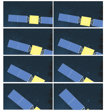
The rotation angles corresponding to the three feature points on the circle are Φ₁=0, Φ₂=π/2, and Φ₃=π. For the relative distance between 3 m and 1 m, points and lines on the target can be observed. While the relative distance is less than 1 m, only four feature points can be observed. Figs. 12-13 show the changes of FOV and features, respectively.

The sampling period, initial state error matrix, measurement noise matrix, and process noise matrix for EKF, and the STF and FASTF are set as follows:

$ T = 0.1{\rm{s}},\mathit{\boldsymbol{R}} = \sigma _{\rm{R}}^2{\mathit{\boldsymbol{I}}_{16}} $

$ {\mathit{\boldsymbol{P}}_0} = {\rm diag}\left( {\sigma _{{P_q}}^2{\mathit{\boldsymbol{I}}_4},\sigma _{{P_p}}^2{\mathit{\boldsymbol{I}}_4},\sigma _{{P_\omega }}^2{\mathit{\boldsymbol{I}}_4},\sigma _{{P_v}}^2{\mathit{\boldsymbol{I}}_4},\sigma _{{P_\mathit{\Phi }}}^2{\mathit{\boldsymbol{I}}_4}} \right) $

$ \mathit{\boldsymbol{Q}} = {\rm diag}\left( {\sigma _{{Q_q}}^2{\mathit{\boldsymbol{I}}_4},\sigma _{{Q_p}}^2{\mathit{\boldsymbol{I}}_4},\sigma _{{Q_\omega }}^2{\mathit{\boldsymbol{I}}_4},\sigma _{{Q_v}}^2{\mathit{\boldsymbol{I}}_4},\sigma _{{Q_\mathit{\Phi }}}^2{\mathit{\boldsymbol{I}}_4}} \right) $

where

$ \begin{array}{*{20}{c}} {\sigma _{{P_q}}^2 = \sigma _{{P_\omega }}^2 = \sigma _{{P_\mathit{\Phi }}}^2 = \sigma _{{Q_q}}^2 = \sigma _{{Q_\omega }}^2 = }\\ {\sigma _{{Q_\mathit{\Phi }}}^2 = \sigma _R^2 = 0.000\;{{01}^2}} \end{array} $

$ \sigma _{{P_p}}^2 = {0.004^2},\sigma _{{P_v}}^2 = {0.04^2} $

$ \sigma _{{Q_p}}^2 = 0.000\;{5^2},\sigma _{{Q_v}}^2 = {0.025^2} $

The forgetting factor ρ=0.98, the parameters set by EKF and the STF are the same as those of FASTF, and the fixed weakening factor of the STF β=1.

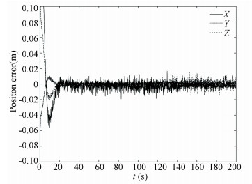
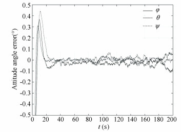
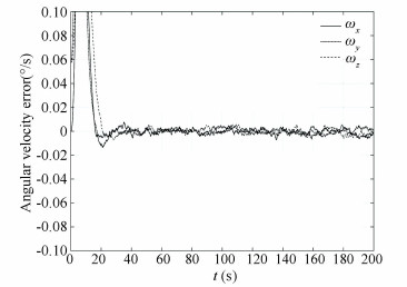
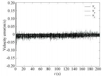
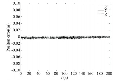
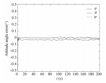
The final approaching time is about 200 s. The simulation results for EKF and STF are presented in Figs. 14-21 for comparison. The estimation errors for the FASTF are shown in Figs. 22-25. The state estimation errors are summarized in Table 3.

The above comparison shows that the STF converges to the reference states within 1.5 s, which is much faster than EKF algorithm converging within 30 s. For the estimation accuracy, EKF converges to 0.015 m and 0.100° for the final 50 s, while the STF converges to about 0.010 m and 0.080°. The convergence speed of the FASTF is approximately the same as that of the STF, but the FASTF converges to much higher values about 0.005 m and 0.030°.The overall performance of the FASTF has the best performance among the three algorithms.

7 Conclusions

The quantity of spacecraft running on orbit is increasing, so it is necessary to develop on-orbit service technology. The accuracy requirement on the relative states between two spacecraft of on-orbit servicing mission is pretty high in the final approaching stage. Considering the integration of attitude and orbit of spacecraft, an accurate relative dynamics model of spacecraft was established by dual quaternion. An FASTF was proposed to overcome the inherent shortcomings of the STF to improve the its tracking performance.The method combined the selection of the weakening factor in the STF with the fuzzy adaptive controller, and realized the adaptive adjustment of the weakening factor and the multiple suboptimal fading matrix, thus improving the filter estimation performance. In future, ground experiment will be designed and carried out to validate the practical precision of the proposed method.