Shape Memory Alloy (SMA) is a special material. Since Greninger and Mooradian[1] observed the shape memory effect on SMA, this material has attracted considerable attention in many scientific fields, such as aerospace[2], aviation[3], and medical application[4]. The characteristic [5-6] and constitutive model [7-8] of SMA were developed in the early 20th century. Subsequently, voluminous literature has focused on the analysis of the solution to SMA model in determinative cases. For an SMA actuator, the analysis results have been proposed[9], which were applied to the field of mechanical design[10]. In view of the two-point distribution technique, the exact solution to SMA's heat exchanger was received[11].
In stochastic cases, the research of probability response is an important topic for nonlinear dynamical systems. In recent years, many methods[12-14] have been developed to solve the problem of probability response, including stochastic averaging method, equivalent nonlinear method[15], and Monte Carlo method. In Ref. [16], super-elastic system's response under white noise excitation was predicted by the Monte Carlo method. However, the Monte Carlo method involves huge amount of computation and complex algorithms. The stochastic averaging method is a powerful approximate technique for the prediction of probability response. Feng[17-18] applied stochastic averaging method to explore the response of Duffing oscillator under white noise. Bifurcation phenomenon is one of the focus topics in dynamical system. In the nonlinear vibro-impact system[19] and SMA system[20], the stochastic averaging method is applied to analyze bifurcation.
Non-smooth factors are widely existent in engineering fields. In previous literature, the methods of non-smooth transformation and stochastic averaging method were rarely studied for the SMA beam model. Thus, this paper focuses on discussing the probability response and bifurcation for the SMA beam model using stochastic averaging method. Section 2 introduces the SMA beam model with rigid constraint. In view of the non-smooth transformation, the stochastic averaging method is carried out to obtain the average Fokker Planck Kolmogorov (FPK) equation in Section 3. Section 4 shows the numerical results to verify the analytical results. Moreover, the critical values of stochastic bifurcation are investigated in detail.
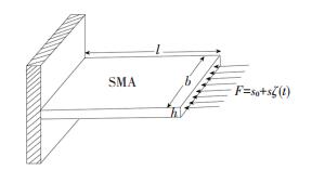
2 Shape Memory Alloy Beam ModelConsider the model of SMA beam[21]with constraint in Fig. 1. l, h, b represent the length, thickness, and width of the beam, respectively. The model is excited by
|
Fig.1 The SMA beam model |
| $ F = {s_0} + s\zeta (t) $ | (1) |
where s0 represents generalized displacement at the initial moment, ζ(t) is the standard Gaussian white noise, and t is time. ζ(t) satisfies
| $ \begin{array}{*{20}{c}} {E[\zeta (t)] = 0}\\ {E[\zeta (t + \tau )\zeta (t)] = \delta (\tau )} \end{array} $ | (2) |
where τ is the time difference, E is the mean, and δ(τ) represents Dirac delta function.
The motion equation for the beam is as follows:
| $ \frac{{{\partial ^2}M}}{{\partial {x^2}}} + F\frac{{{\partial ^2}\omega }}{{\partial {x^2}}} + c\frac{{\partial \omega }}{{\partial t}} + \rho A\frac{{{\partial ^2}\omega }}{{\partial {t^2}}} = 0 $ | (3) |
where M is bending moment of the beam, c represents linear damping, ω is lateral displacement of the beam, and ρA is the mass of the beam per unit length.
Then, the stochastic nonlinear motion equation of SMA beam can be expressed as
| $ \ddot x - kx + \alpha {x^3} + \left( {\tilde \mu - \tilde \gamma {x^2} + \tilde \beta {{\dot x}^2}} \right)\dot x = \tilde f\zeta (t) $ | (4) |
where
| $ k = {{\rm{ \mathsf{ π} }}^4} - \frac{{{s_0}{{\rm{ \mathsf{ π} }}^2}}}{{{a_1}{I_1}}},\alpha = \frac{{3{a_3}{I_3}{{\rm{ \mathsf{ π} }}^8}}}{{4{a_1}{I_1}}},\tilde \mu = \frac{{cl}}{{{{\left[ {\rho A{a_1}{I_1}} \right]}^{1/2}}}} $ |
| $ \tilde \gamma = \frac{{3{a_5}{I_3}{{\rm{ \mathsf{ π} }}^8}}}{{4{{\left[ {\rho A{a_1}{I_1}} \right]}^{1/2}}l}},\tilde \beta = \frac{{{c^2}{l^2}}}{{\rho A{a_1}{I_1}}} $ |
| $ \tilde f = \frac{{4{l^2}}}{{{a_1}{I_1}{\rm{ \mathsf{ π} }}}},{I_1} = \frac{{b{h^3}}}{{12{l^2}}},{I_3} = \frac{{b{h^5}}}{{80{l^6}}} $ |
| $ {a_1} = {b_1} + 3{b_2}\varepsilon _0^2,{a_3} = {b_2},{a_5} = \frac{a}{{\varepsilon _0^2}} $ |
ε0 is the symmetric center of the ring, and s represents generalized displacement.
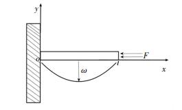
Fig. 2 shows the sectional view of the model. The dimensionless equation of motion is
|
Fig.2 Sectional view of the beam with one-side rigid constraint |
| $ \left\{ {\begin{array}{*{20}{l}} {\ddot x - kx + \alpha {x^3} + \left( {\tilde \mu - \tilde \gamma {x^2} + \tilde \beta {{\dot x}^2}} \right)\dot x = \tilde f\zeta (t),x > 0}\\ {{{\dot x}_ + } = - R{{\dot x}_ - },x = 0} \end{array}} \right. $ | (5) |
where k, α,
Non-smooth transformation is introduced[22-25]:
| $ \begin{array}{*{20}{c}} {x = {x_1} = |y| + \Delta ,\dot x = {x_2} = \dot y\text{sgn}(y)}\\ {\ddot x = \ddot y\text{sgn}(y),\text{sgn}(y) = \left\{ {\begin{array}{*{20}{r}} {1,y > 0}\\ { - 1,y < 0} \end{array}} \right.} \end{array} $ | (6) |
With Δ=0 and Eq.(6), Eq.(5) can be rewritten as
| $ \begin{array}{*{20}{c}} {\ddot y - ky + \alpha {y^3} + \left( {\tilde \mu - \tilde \gamma {y^2} + \tilde \beta {{\dot y}^2}} \right)\dot y + }\\ {(1 - R)\dot y|\dot y|\delta (y) = \tilde f \text{sgn} (y)\zeta (t)} \end{array} $ | (7) |
where δ(y) is Dirac delta function.
Compare the energy difference between the stochastic excitation and the damp. If system energy is powerful within a period, Eq.(7) can be regarded as a quasi-conservative system. Assume
| $ \left\{ {\begin{array}{*{20}{l}} {{{\dot y}_1} = {y_2}}\\ {{{\dot y}_2} = k{y_1} - \alpha y_1^3 - \varepsilon \left( {\mu - \gamma y_1^2 + \beta y_2^2} \right){y_2} - }\\ {\;\;\;\;\;(1 - R){y_2}\left| {{y_2}} \right|\delta \left( {{y_1}} \right) + \sqrt \varepsilon f \text{sgn} \left( {{y_1}} \right)\zeta (t)} \end{array}} \right. $ | (8) |
Using the Itô formula, Eq.(8) is reduced to the following Itô differential equation:
| $ \left\{ {\begin{array}{*{20}{l}} {{\rm{d}}{y_1} = {y_2}{\rm{d}}t}\\ {{\rm{d}}{y_2} = \left[ {k{y_1} - \alpha y_1^3 - \varepsilon \left( {\mu - \gamma y_1^2 + \beta y_2^2} \right){y_2} - } \right.}\\ {\left. {\left( {1 - R} \right){y_2}\left| {{y_2}} \right|\delta \left( {{y_1}} \right) + \frac{1}{2}\varepsilon {f^2}y_1^2} \right]{\rm{d}}t + }\\ {\sqrt \varepsilon f \text{sgn} \left( {{y_1}} \right){\rm{d}}W(t)} \end{array}} \right. $ | (9) |
in which W(t) is the Wiener process.
When ε=0 in Eq.(8), the unperturbed system is obtained. The corresponding energy function and potential function are
| $ H = \frac{{y_2^2}}{2} - \frac{k}{2}y_1^2 + \alpha \frac{{y_1^4}}{4} $ | (10) |
| $ U\left( {{y_1}} \right) = - \frac{k}{2}y_1^2 + \alpha \frac{{y_1^4}}{4} $ | (11) |
The derivative of the energy Eq.(10) on the time t is
| $ \begin{array}{l} \dot H = {y_2}\left[ { - \varepsilon \left( {\mu - \gamma y_1^2 + \beta y_2^2} \right){y_2} - (1 - } \right.\\ \;\;\;\;\;\;\left. {R){y_2}\left| {{y_2}} \right|\delta \left( {{y_1}} \right) + \sqrt \varepsilon f \text{sgn} \left( {{y_1}} \right)\zeta (t)} \right] \end{array} $ | (12) |
According to the Itô formula, the Itô stochastic differential equation of Eq. (12) can be expressed as
| $ \begin{array}{l} {\rm{d}}H = \left[ {{y_2}\left[ { - \varepsilon \left( {\mu - \gamma y_1^2 + \beta y_2^2} \right){y_2} - } \right.} \right.\\ \;\;\;\;\;\;\;\;\left. {\left. {(1 - R){y_2}\left| {{y_2}} \right|\delta \left( {{y_1}} \right)} \right] + \frac{1}{2}\varepsilon {f^2}} \right]{\rm{d}}t + \\ \;\;\;\;\;\;\;\;\sqrt \varepsilon f{y_2} \text{sgn} \left( {{y_1}} \right){\rm{d}}W(t) \end{array} $ | (13) |
It is known from the Khassminskii theorem[26], y1 and y2 are two fast mutative processes, and H(t) is a slow mutative process, which is approach to a Markov process as ε→0. Therefore, the averaging Itô stochastic diffusion process of the Markov process can be described as
| $ {\rm{d}}H = \langle m(H)\rangle {\rm{d}}t + \langle \sigma (H)\rangle {\rm{d}}W(t) $ | (14) |
where W(t) is the Wiener process, 〈m(H)〉 and 〈σ(H)〉 are the mean drift and mean diffusion coefficients:
| $ \begin{array}{l} \langle m(H)\rangle = \frac{1}{{{T_{\frac{1}{4}}}(H)}}[ - \varepsilon \mu B(H) + \varepsilon \gamma S(H) - \\ \;\;\;\;\;\;\;\;\;\;\;\;\;\;\left. {\varepsilon \beta Q(H) + (R - 1)H + \frac{1}{2}\varepsilon {f^2}{T_{\frac{1}{4}}}(H)} \right] \end{array} $ | (15) |
| $ \left\langle {{\sigma ^2}(H)} \right\rangle = \frac{{\varepsilon {f^2}}}{{{T_{\frac{1}{4}}}(H)}}B(H) $ | (16) |
| $ \begin{array}{l} {T_{\frac{1}{4}}}(H) = \frac{{T(H)}}{4} = \int_0^A {\frac{1}{{\sqrt {2H - 2U\left( {{y_1}} \right)} }}{\rm{d}}{y_1}} = \\ \;\;\;\;\;\;\;\;\;\;\;\;\;\frac{1}{{\sqrt {\alpha {A^2} - k} }}{E_1}(K) = \frac{1}{{\sqrt M }}{E_1}(K) \end{array} $ |
| $ B(H) = \frac{{2\sqrt M }}{{3\alpha }}\left[ {(M - N){E_1}(K) + (2N - M){E_2}(K)} \right] $ |
| $ \begin{array}{l} S(H) = \frac{{4\sqrt M }}{{15{\alpha ^2}}}\left[ {\left( {3MN - 2{M^2} - {N^2}} \right){E_1}(K) + } \right.\\ \;\;\;\;\;\;\;\;\;\;\;\;\left. {2\left( {{M^2} + {N^2} - 2MN} \right){E_2}(K)} \right] \end{array} $ |
| $ \begin{array}{l} Q(H) = \frac{{4\sqrt M }}{{35{\alpha ^2}}}\left[ {\left( {8{N^3} - 13M{N^2} + 3{M^2}N + 2{M^3}} \right){E_1}(K) + } \right.\\ \;\;\;\;\;\;\;\;\;\;\;\;\left. {2\left( { - 8{N^3} + 12M{N^2} - 2{M^2}N - {M^3}} \right){E_2}(K)} \right] \end{array} $ |
| $ M = \alpha {A^2} - k,N = \frac{{\alpha {A^2}}}{2},K = \frac{N}{M} $ |
where E1(K), E2(K) are the first and second kind of complete elliptic integrals, respectively, and
| $ {E_1}(K) = \int_0^{\frac{{\rm{ \mathsf{ π} }}}{2}} {\frac{1}{{\sqrt {1 - K{{\sin }^2}\theta } }}{\rm{d}}\theta } $ |
| $ {E_2}(K) = \int_0^{\frac{\pi }{2}} {\sqrt {1 - K{{\sin }^2}\theta } {\rm{d}}\theta } $ |
where A is the positive root of equation U(A) =H. Thus, combination with Eq.(11) obtains the following equation:
| $ A = \sqrt {\frac{{\sqrt {{k^2} + 4\alpha H} + k}}{\alpha }} $ | (17) |
The average FPK equation of Eq.(14) is
| $ \frac{{\partial p}}{{\partial t}} = - \frac{\partial }{{\partial H}}\left[ {\langle m(H)\rangle p} \right] + \frac{1}{2}\frac{{{\partial ^2}}}{{\partial H}}\left[ {\left\langle {{\sigma ^2}(H)} \right\rangle p} \right] $ | (18) |
where p represents the probability density function (PDF) of energy function H.
The steady state solution implies
| $ \left\{ {\begin{array}{*{20}{l}} {0 \le p < \infty ,\quad H = 0}\\ {p \to 0,\frac{{{\rm{d}}p}}{{{\rm{d}}H}} \to 0,H \to \infty } \end{array}} \right. $ | (19) |
Therefore, the steady state solution of slow variable H can be described as
| $ p(H) = {C_0}\exp [ - \lambda (H)] $ | (20) |
where
| $ \begin{array}{l} \lambda (H) = - 2\int_0^H {\frac{{ - \mu B(x) + \gamma C(x) - \beta Q(x) + (R - 1)x}}{{B(x)}}{\rm{d}}x} - \\ \;\;\;\;\;\;\;\;\;\;\ln \frac{{{T_{\frac{1}{4}}}(H)}}{{{T_{\frac{1}{4}}}(0)}} \end{array} $ | (21) |
and C0 is a normalized constant. The joint PDF of Eq.(5) can be obtained as below:
| $ \begin{array}{l} p\left( {{x_1},{x_2}} \right) = {p_{{y_1}{y_2}}}\left( {{y_1},{y_2}} \right)\left| {\frac{{\partial \left( {{y_1},{y_2}} \right)}}{{\partial \left( {{x_1},{x_2}} \right)}}} \right| = \\ \;\;\;\;\;\;\;{{\tilde p}_{{y_1}{y_2}}}\left( {{x_1},{x_2}} \right) + {{\tilde p}_{{y_1}{y_2}}}\left( { - {x_1}, - {x_2}} \right) = \\ \;\;\;\;\;\;\;2{{\tilde p}_{{y_1}{y_2}}}\left( {{x_1},{x_2}} \right) = {\left. {2\frac{{p(H)}}{{T(H)}}} \right|_{H = \frac{{y_2^2}}{2} - \frac{k}{2}y_1^2 + \alpha \frac{{y_1^4}}{4}}} \cdot \\ \;\;\;\;\;\;\;\left| {\frac{{\partial \left( {{y_1},{y_2}} \right)}}{{\partial \left( {{x_1},{x_2}} \right)}}} \right|,{x_1} \ge 0 \end{array} $ | (22) |
The edge PDFs are received from Eq.(22):
| $ p\left( {{x_1}} \right) = \int_{ - \infty }^{ + \infty } p \left( {{x_1},{x_2}} \right){\rm{d}}{x_2} $ | (23) |
| $ p\left( {{x_2}} \right) = \int_{ - \infty }^{ + \infty } p \left( {{x_1},{x_2}} \right){\rm{d}}{x_1} $ | (24) |
In this section, the system parameters are taken as k=-1.0, α=0.01, γ=0.01, β=0.01. Based on the original Eq.(5), the numerical results can be obtained by Monte Carlo method. Moreover, stochastic bifurcations is discussed.
4.1 Numerical SimulationThe influence of restitution coefficient R and noise amplitude f on the probability responses of Eq.(5) is considered. Let the parameter μ be 0.01 in this subsection.
As illustrated in Fig. 3, it is obvious that analytical results agree with numerical results. When noise amplitude is fixed, the smaller restitution coefficient R could lead to higher peaks of PDFs p(H), displacement p(x1), and velocity p(x2). In addition, Fig. 3(a), (b), and (c) show that the influence of noise amplitude f is similar to restitution coefficient R. These results indicate that the smaller restitution value can make the larger loss of energy, and stochastic perturbation can result in the system's deviation from the equilibrium position.

|
Fig.3 Analytical results and numerical results of Eq.(5) for different R and f |
4.2 Stochastic Bifurcations
In this subsection, the noise amplitude f is fixed as 0.1. The effect of linear damping coefficient μ and restitution coefficient R on PDFs of Eq.(5) were explored.
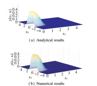
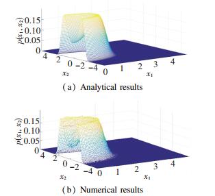
It can be seen from Figs. 4-5, analytical results agree well with numerical results when μ=-0.01. When R=0.98, a single peak appears in the joint PDFs as shown in Fig. 4. As the restitution coefficient R increases to 1.0, the join PDFs transits to the shape of crater. This change of PDFs implies that Eq.(5) undergoes a P-bifurcation.
|
Fig.4 Joint PDFs of Eq.(5) when R =0.98 |
|
Fig.5 Joint PDFs of Eq.(5) when R =1.0 |
To discover the detailed process of P-bifurcation, the curve of the edge PDFs for different restitution coefficient R is shown in Fig. 6.

|
Fig.6 The edge PDFs of Eq.(5) for different restitution coefficient R |
Obviously, there is only a singular peak for R=0.98. As restitution coefficient R increases, the curve becomes flatter and eventually turns into a crater for R=1.0. It is can be seen in Fig. 6 that the critical value is about R≈0.993 during transition. On the other hand, the evolution of edge PDFs implies that a smaller R can cause a larger loss of energy.
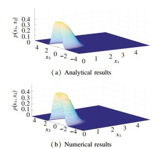
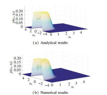
Comparison of Fig. 7 and Fig. 8 shows that analytical results coincide with numerical results well. As μ decreases from -0.01 to -0.02, the curve changes from single peak to a crater. The changes indicate the occurrence of P-bifurcation.
|
Fig.7 Joint PDFs of Eq.(5) when μ =-0.01 |
|
Fig.8 Joint PDFs of Eq.(5) when μ =-0.02 |
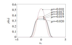
For different linear damping coefficients μ, Fig. 9 describes the procedure of P-bifurcation in detail. It is easy to see one peak occurs for μ=-0.01. As μ decreases, the curve gets increasingly flatter. Finally, when μ=-0.02, the form of crater appears. From the evolution of edge PDFs, it was found that μ≈-0.018 was the critical value that made stochastic bifurcation happen.
|
Fig.9 The edge PDFs of Eq. (5) for different linear damping coefficients μ |
5 Conclusions
In this paper, the probability response of SMA impact model under external Gaussian white noise excitation is investigated. First, the non-smooth transformation was employed to deal with the discontinuous position. Then the original system turned into an approximate system associated with the Dirac function. Lastly, the stochastic response of the approximate system was obtained after analysis. Meanwhile, comparison of analytical results with numerical results demonstrates the effectiveness of the stochastic averaging method. It reveals that the stationary probability response of system is affected by the increase of noise amplitude and restitution force.
Furthermore, this paper explores the P-bifurcation of SMA beam system. It is worth noting that the restitution coefficient R and linear damping coefficient μ can cause P-bifurcation. However, the P-bifurcation usually results in transition of dynamical system, in which unstable vibration is generated and the stability of the SMA beam is destroyed. Therefore, by adjusting the system parameters, the security of the SMA beam could be enhanced.
| [1] |
Greninger A B, Mooradian V G. Strain transformation in metastable beta copper-zinc and beta copper-tin alloys. Transactions of the Metallurgical Society of AIME, 1938, 128: 337. (  0) 0) |
| [2] |
Cao D Q, Shao C H, Xu Y Q, et al. Aero-elastic flutter characteristics of laminated composite panel embedded with shape memory alloy wires. Journal of Harbin Institute of Technology (New Series), 2017, 24(5): 32-38. DOI:10.11916/j.issn.1005-9113.16049 (  0) 0) |
| [3] |
Zhou B, Leng J S, Zou G P, et al. Constitutive model for shape memory alloy torsion actuator. Journal of Harbin Institute of Technology (New Series), 2010, 17(2): 278-282. DOI:10.11916/j.issn.1005-9113.2010.02.024 (  0) 0) |
| [4] |
Khalil-Allafi J, Amin-Ahmadi B, Zare M. Biocompatibility and corrosion behavior of the shape memory NiTi alloy in the physiological environments simulated with body fluids for medical applications. Materials Science and Engineering: C, 2010, 30(8): 1112-1117. DOI:10.1016/j.msec.2010.06.007 (  0) 0) |
| [5] |
Brinson L C. One-dimensional constitutive behavior of shape memory alloys: Thermomechanical derivation with non-constant material functions and redefined martensite internal variable. Journal of Intelligent Material Systems and Structures, 1993, 4(2): 229-242. DOI:10.1177/1045389X9300400213 (  0) 0) |
| [6] |
Raboud D. Simulation of the super-elastic Response of SMA orthodontic wires. Journal of Biomechanical Engineering, 1998, 120(5): 676-685. DOI:10.1115/1.2834761 (  0) 0) |
| [7] |
Seelecke S. Modeling the dynamic behavior of shape memory alloys. International Journal of Non-Linear Mechanics, 2002, 37(8): 1363-1374. DOI:10.1016/S0020-7462(02)00030-6 (  0) 0) |
| [8] |
Wang L X, Melink R V N. Numerical model for vibration damping resulting from the first-order phase transformations. Applied Mathematical Modeling, 2007, 31(9): 2008-2018. DOI:10.1016/j.apm.2006.08.019 (  0) 0) |
| [9] |
Peng J S, Yang L, Luo G B, et al. Nonlinear electro-dynamic analysis of micro-actuators: Effect of material nonlinearity. Applied Mathematical Modeling, 2014, 38(11-12): 2781-2790. DOI:10.1016/j.apm.2013.10.070 (  0) 0) |
| [10] |
Majima S, Kodama K, Hasegawa T. Modeling of shape memory alloy actuator and tracking control system with the model. IEEE Transactions on Control Systems Technology, 2001, 9(1): 54-59. DOI:10.1109/87.896745 (  0) 0) |
| [11] |
Prasad R C, Karmeshu, Bharadwaj K K. Stochastic modeling of heat exchanger response to data uncertainties. Applied Mathematical Modeling, 2002, 26(6): 715-726. DOI:10.1016/S0307-904X(01)00082-8 (  0) 0) |
| [12] |
Roberts J B, Spanos P D. Stochastic averaging: An approximate method of solving random vibration problems. International Journal of Non-Linear Mechanics, 1986, 21(2): 111-134. DOI:10.1016/0020-7462(86)90025-9 (  0) 0) |
| [13] |
Bouc R. The power spectral density of response for a strongly non-linear random oscillator. Journal of Sound and Vibration, 1994, 175(3): 317-331. DOI:10.1006/jsvi.1994.1331 (  0) 0) |
| [14] |
Red-Horse J R, Spanos P D. A generalization to stochastic averaging in random vibration. International Journal of Non-Linear Mechanics, 1992, 27(1): 85-101. DOI:10.1016/0020-7462(92)90025-3 (  0) 0) |
| [15] |
Yan X J, Nie J X. Prediction of the response of SMA superelastic systems under stationary random excitation. Journal of Beijing University of Aeronautics and Astronautics, 2001, 27(6): 690-693. DOI:10.13700/j.bh.1001-5965.2001.06.019 (  0) 0) |
| [16] |
Yan X, Nie J. Response of SMA super-elastic system under random excitation. Journal of Sound and Vibration, 2000, 238(5): 893-901. DOI:10.1006/jsvi.2000.3020 (  0) 0) |
| [17] |
Feng J Q, Xu W, Rong H W, et al. Stochastic responses of Duffing-Van der Pol vibro-impact system under additive and multiplicative random excitations. International Journal of Non-Linear Mechanics, 2009, 44(1): 51-57. DOI:10.1016/j.ijnonlinmec.2008.08.013 (  0) 0) |
| [18] |
Feng J Q, Xu W, Wang R. Stochastic responses of vibro-impact duffing oscillator excited by additive Gaussian noise. Journal of Sound and Vibration, 2008, 309(3-5): 730-738. DOI:10.1016/j.jsv.2007.07.070 (  0) 0) |
| [19] |
Yang Y G, Xu W, Sun Y H, et al. Stochastic bifurcations in the nonlinear vibroimpact system with fractional derivative under random excitation. Communications in Nonlinear Science and Numerical Simulation, 2017, 42: 62-72. DOI:10.1016/j.cnsns.2016.05.004 (  0) 0) |
| [20] |
Yu Y, Zhang Z D, Bi Q S, et al. Bifurcation analysis on delay-induced bursting in a shape memory alloy oscillator with time delay feedback. Applied Mathematical Modeling, 2016, 40(3): 1816-1824. DOI:10.1016/j.apm.2015.09.010 (  0) 0) |
| [21] |
Ge G, Zhu Z W, Xu J. Chaotic and safe basin erosion of shape memory alloy beam under combined excitation of simple harmonic and white noise. Journal of Vibration and Shock, 2012, 31(23): 2-11. DOI:10.13465/j.cnki.jvs.2012.23.009 (  0) 0) |
| [22] |
Zhu Z W, Zhang Q X, Xu J. Nonlinear dynamic characteristics and optimal control of a giant magneto-strictive film-shaped memory alloy composite plate subjected to in-plane stochastic excitation. Chinese Physics B, 2014, 23(8): 169-175. DOI:10.1088/1674-1056/23/8/088201 (  0) 0) |
| [23] |
Feng J Q. Nonlinear Dynamics of a Typical Collisional Vibration System. Beijing: Science Press, 2018: 64-84.
(  0) 0) |
| [24] |
Dimentberg M F, Iourtchenko D V. Random vibrations with impacts: A review. Nonlinear Dynamics, 2004, 36(2-4): 229-254. DOI:10.1023/B:NODY.0000045510.93602.ca (  0) 0) |
| [25] |
Zhuravlev V F. A method for analyzing vibration-impact systems by means of special functions. Mechanics of Solids, 1976, 2: 23-27. (  0) 0) |
| [26] |
Zhu W Q. Nonlinear Stochastic Dynamics and Control. Beijing: Science Press, 2003: 203-270.
(  0) 0) |
 2020, Vol. 27


