2. Institute of Robotics and Intelligent Systems, Wuhan University of Science and Technology, Wuhan 430081, China
In the field of service robotics, autonomous robots are required to complete the tasks of family service[1], elderly escort, and scene monitoring independently in indoor environments[2], where indoor localization technology is a prerequisite.
Monte Carlo localization (MCL) algorithm was first proposed in 1999 in Ref. [3], which is obtained by substituting the appropriate probabilistic motion and perception model into the particle filter[4]. The MCL algorithm uses a large number of particles to represent the confidence of the robot's position. The measurement model determines the importance weight of the particle, and then samples the particle that can represent the position of the robot from the motion model. Although the MCL method can deal with global localization, the "kidnapped problem" or global localization loss is still an issue, which is the situation when a well-tracked robot suddenly moves to somewhere else without being told during an interior mission[5]. Once such a situation occurs, the robot may execute a wrong action using wrong information, which will damage the environment or hurt itself. The "kidnapped problem" is a complex variant of the global localization. The practical significance of this issue comes from the observation of the most advanced localization algorithms. However, current algorithms are not always stable, so it is essential for robots to possess the ability to recover from localization loss by themselves[6]. To solve the problem of robot localization loss and "kidnapped problem", foreign and domestic scholars have achieved some results in the research of two-dimensional map[7], three-dimensional map[8-9], and localization based on ROS[10-11]. Scholars from China Central South University proposed an improvement algorithm named Adaptive Monte Carlo localization (AMCL) for multi-hypothesis tracking[12]. Based on particle clustering, the algorithm can reduce the impact of "kidnapping" on robots by reducing particle degradation. He[13] proposed a self-localization algorithm based on genetic algorithm. By introducing divergence parameters, the algorithm can maintain particle diversity and reduce the particle deprivation effect to make localization more accurate, which allows the robot to have the specific ability to recover when it is "kidnapped." Scholars from Ritsumeikan University[14] proposed an algorithm for detecting and identifying double "kidnapping problems". Further analyses detected the existence of "kidnapping problems" and analyzed them in Ref. [15] only when it is under conditions that are better resolved in Ref. [16]. Since the indoor environment is complex and diverse, the "kidnapping problem" is different.
Although many scholars have improved methods to solve the "kidnapping problem", few have discussed the exhaustive analysis of various positioning failures and the corresponding solutions. In this paper, an improved MCL (IMCL) algorithm is proposed on the basis of the existing MCL with the combination of the characteristics of particle resampling and the analysis of different situations of localization loss. When a robot is under the condition of positioning failure, different particle sampling methods can help it to recover its positioning function. The theoretical analysis and experimental verification of the invalidation of the robot are performed in this paper to verify the effectiveness of the proposed algorithm.
2 IMCL Algorithm 2.1 Theoretical BackgroundThe AMCL algorithm is a further improvement of the MCL algorithm[17]. By tracking the likelihood p=(zk|z1:k-1, u1:k, m) of the short-term likelihood (wfast) and the long-term likelihood (wslow) of the likelihood value, the resampling random divergence is dynamically adjusted based on changes in likelihood[18]. When the robot is in the "kidnapping" state, the short-term likelihood (wfast) falls faster than the long-term likelihood (wslow), and the resampling increases the diversity of new particles based on the difference[19]. Although the AMCL algorithm will generate new particles, it cannot solve the robot's "kidnapping problem" due to its limitations which can be effectively solved by the IMCL algorithm proposed in this paper.
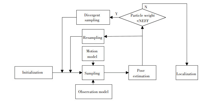
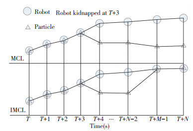
When the robot is in the "kidnapping" state, the matching degree between the environment of the observed robot and the actual map environment will decrease, which will affect the weights of the sample particles. The controller can then judge whether the robot is in the "kidnapping" state by changing the weight. In this way, a self-recovery localization mechanism is used to help the robot relocate. The process of the localization is shown in Fig. 1 and the comparison of the MCL and IMCL relocalization processes is shown in Fig. 2.
|
Fig.1 Flowchart of localization |
|
Fig.2 Comparison of MCL and IMCL relocalization processes |
Initialization is introduced to represent the robot's possible position on the grid map by scattering particles. According to the distance information returned by the laser radar, the direction information returned by the gyroscope, and the displacement information carried by the encoder, the sampling of the particles is completed and the particles that can represent the real position of the robot can thus be obtained. The key step is divergent sampling that when the robot fails localization due to hardware or artificial displacement, it is necessary to generate new particles that can represent the real position of the robot through divergent sampling.
2.2 Derivation of IMCL Algorithm TheoryThe main idea of the IMCL is to introduce divergent sampling.The purpose of robot localization is to obtain the real-time state of the robot. The solving recursive equations are expressed as follows:
| $ p\left( {{x_k}{\text{|}}{z_{1:k}}} \right) = \frac{{p\left( {{z_k}{\text{|}}{x_k}} \right)p\left( {{x_k}{\text{|}}{z_{1:k - 1}}} \right)}}{{p\left( {{z_k}{\text{|}}{z_{1:k - 1}}} \right)}} $ | (1) |
For nonlinear systems, the analytical solution of this formula does not exist or is difficult to obtain.
Posterior distributed (M) particles can be expressed as
| $ {x_k}: = x_k^1, x_k^2, \ldots , x_k^m $ | (2) |
where the confidence
| $ {\text{bel}}\left( {{x_{0:k}}} \right) = p({x_{0:k}}|{u_{1:k}}, {z_{1:k}}) $ | (3) |
and specifically
| $ \begin{array}{*{20}{l}} {p\left( {{x_{0:k}}|{z_{1:k}}, {u_{1:k}}} \right) = } \\ {\eta p\left( {{z_k}|{x_{0:k}}, {z_{1:k - 1}}, {u_{1:k}}} \right)p\left( {{x_{0:k}}|{z_{1:k - 1}}, {u_{1:k}}} \right) = } \\ {\eta p\left( {{z_k}|{x_k}} \right)p\left( {{x_{0: k}}|{z_{1:k - 1}}, {u_{1:k}}} \right) = } \\ {\eta p\left( {{z_k}|{x_k}} \right)p\left( {{x_k}|{x_{0:k - 1}}, {z_{1:k - 1}}, {u_{1:k}}} \right) \cdot } \\ {p\left( {{x_{0:k - 1}}|{z_{1:k - 1}}, {u_{1:k}}} \right) = } \\ {\eta p\left( {{z_k}|{x_k}} \right)p\left( {{x_k}|{x_{k - 1}}, {u_k}} \right) \cdot } \\ {p\left( {{x_{0:k - 1}}|{z_{1:k - 1}}, {u_{1:k - 1}}} \right)} \end{array} $ | (4) |
During solving process, the robot uses the state estimation value at time step k-1 and the control amount uk from time step k-1 to time step k to obtain the state transition distribution P(xk|uk, xk-1) through the motion model. The estimated state xkm at time step k from random sampling in the state transition distribution is thus obtained.
By comparing the map information contained in the observation model of each particle, the matching degree of each particle and the position of robot (xk, yk, θk) are obtained, that is, the weight wk[m] of the information is represented by particles (x, y, θ).
| $ w_k^{[m]} = {\text{measurement}}\_{\text{model}}\left( {{z_k}, x_k^{[m]}, m} \right) $ | (5) |
| $ \begin{array}{l} w_k^{[m]} = \frac{{{\text{ Target distribution }}}}{{{\text{ Proposal distribution }}}} = \hfill \\ \;\;\;\frac{{\eta p\left( {{z_k}|{x_k}} \right)p\left( {{x_k}|{x_{k - 1}}, {u_k}} \right)p\left( {{x_{0:k - 1}}|{z_{1:k - 1}}, {u_{1:k - 1}}} \right)}}{{p\left( {{x_k}|{x_{k - 1}}, {u_k}} \right)p\left( {{x_{0:k - 1}}|{z_{0:k - 1}}, {u_{0:k - 1}}} \right)}} = \hfill \\ \;\;\;\eta p\left( {{z_k}|{x_k}} \right) \hfill \\ \end{array} $ | (6) |
The probability of resampling particles is proportional to the weight wk[m], and the particles produced by the resampling are distributed according to the product of the proposed distribution and the weight wk[m].
| $ \begin{array}{l} {\text{bel}}\left( {{x_{0:k}}} \right) = \eta w_k^mp\left( {{x_k}|{x_{k - 1}}, {u_k}} \right)p({x_{0:k - 1}}|{z_{1:k - 1}}, \hfill \\ \;\;\;\;\;\;\;\;\;\;\;\;\;\;\;\;{u_{1:k - 1}}) \hfill \\ \end{array} $ | (7) |
When robot localization is completed, p(xk|z1:k, u1:k) will maintain a high value, but when the robot is in the "kidnapping" state, p(xk|z1:k, u1:k) will suddenly drop and the dynamic Bayesian network recursion will be in an invalid state as follows:
| $p\left( {{x_k}|{z_{1:k}}, {u_{1:k}}} \right) \propto 0 $ | (8) |
| $ {\text{bel}}\left( {{x_{0:k}}} \right) \propto 0\;{\text{or}}\;p\left( {{x_k}|{z_{1:k}}, {u_{1:k}}} \right) < {\text{neff}} $ | (9) |
At this point, the particles are in a degenerate state, so the position information carried by the particles cannot represent the real position of the robot.
If new particles are simply resampled from xk:=xk1, xk2, …, xkm, the position information carried by the particles in the new particles xk+1:=xk+11, xk+12, ..., xk+1m generated by sampling cannot represent the real position of the robot. As a result, the robot will perform erroneous operations based on erroneous information, which is detrimental for itself. Relocalization requires changing the particle sample so more new particles should be included in the sample to represent the robot's position.
When the robot is in alocalization loss or a "kidnapping" state, the AMCL algorithm will generate random particles in the map, which will increase the computational burden on the computer and is inefficient for relocalization. Although random particles are generated, they cannot represent the real position of the robot and will be iterated during the random sampling process, resulting in a state that the robot is still in the initial position loss.
However, the proposed IMCL algorithm associates the generated random particles with the observations of the robot, detects the changes in the weights of the particles, and controls the number of random particles at all times. The new particles will slowly move close to the high-weight particles and iterate at any time so more and more particles will represent the robot's real position.
Assuming that the robot is in alocalization loss at time k, and according to sampling xk:=xk1, xk2, …, xkm, the robot localization will definitely fail that once positioned, the robot will perform the task in a wrong place, which is meaningless.
When the robot k+1 moments move (dx, dy, dθ), then in the AMCL algorithm, the particle motion produces the particle sample set at time k+1 as follows:
| $ {(x_{k + 1}^1, x_{k + 1}^2, \ldots , x_{k + 1}^m)^{\text{T}}} = {\left( {x_k^1, x_k^2, \ldots , x_k^m} \right)^{\text{T}}} + \left( {{d_x}, {d_y}, {d_\theta }} \right) $ | (10) |
From the generated particle sample set, particles are sampled and the robot is still in a loss state.
The IMCL is proposed to change the sample set xk:=xk1, xk2, …, xkm after the fixed localization loss, the robot is in motion, whether in the process of rotation or translational motion, then the IMCL will match iteratively through the motion model and the observation model.
In the process of matching iterations, the weights of the particles are constantly changing and the state of the robot can be determined by detecting this change, which requires the robot to be able to detect the state of the robot by itself. Thus we need to use relevant parameters of the robot as bases to determine whether the robot is in a localization loss state.
Based on previous research, it has been found that there is no change in the weight of the normalized particles that can be used to determine the state of the robot. When the robot is in a localization loss, the sample set of particles can be well changed by the divergent sampling, so that more highly weighted particles are generated.
When the robot k+1 move (dx, dy, dθ) at a time in the IMCL algorithm, the particle motion produces the particle sample set at time k+1 as follows:
| $ \begin{array}{l} (x_{k + 1}^1, x_{k + 1}^2, \ldots , x_{k + 1}^m) = \left( {x_k^1, x_k^2, \ldots , x_k^m} \right) + ({\text{ran}}{{\text{d}}_x}, \hfill \\ \;\;\;\;\;\;\;\;\;\;\;\;\;\;\;\;\;\;\;\;\;\;\;\;\;\;\;\;\;\;\;\;{\text{ran}}{{\text{d}}_y}, {\text{ran}}{{\text{d}}_\theta }) \hfill \\ \end{array} $ | (11) |
| $ \begin{array}{l} {\text{new}}(x_{t + 1}^1, {\text{ }}x_{t + 1}^2, \ldots , x_{t + 1}^m) = (x_{t + 1}^1, {\text{ }}x_{t + 1}^2, \ldots , x_{t + 1}^m)*D\% + \hfill \\ \;\;\;\;\;\;\;\;{\text{rand}}(x_{t + 1}^1, {\text{ }}x_{t + 1}^2, \ldots , x_{t + 1}^m)*\left( {1 - D\% } \right) \hfill \\ \end{array} $ | (12) |
where the D value represents the status of robot localization loss and it will adopt adaptive changes according to different situations of localization losses.
In order to ensure the feasibility and efficiency of the algorithm, multiple sets of correlation parameters are used to determine the loss situation and to ensure that the program does not fall into a local optimum when running. At the same time, the classification of different localization losses can speed up the efficiency of particle optimization.
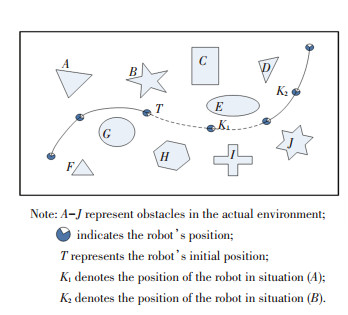
3 Classification of Localization LossesSituations of localization loss can be divided into following types as shown in Fig. 3.
|
Fig.3 Various situations of robot localization loss |
Situation (A): The robot is "kidnapped" near the real localization;
Situation (B): The robot is "kidnapped" far away from the real localization;
(B1): The characteristics of the nearby environment are different;
(B2): The characteristics of the nearby environment are similar.
When the robot is in a localization loss, the average weight of the particles will decrease and the magnitude of the decline in different situations will be different. When the robot is in the loss under situation (A), the weight of the particles that represents the position of the robot will quickly drop to a lower value. Compared with situation (A), the weight of the particles in situation (B) will decrease by a large margin closed to zero. Situation (B) can be divided into similar situation (B1) and dissimilar situation (B2). There are many similar features in a similar environment which makes the data association more complex and the relocalization more difficult.
4 Localization Simulation and Experimental Data Analysis 4.1 Simulation Analysis of LocalizationIn order to verify the effectiveness of the proposed algorithm, this paper establishes the positioning and "kidnapping" of the robot in a simulation environment, in which the IMCL algorithm is verified by comparing the experimental data of IMCL and AMCL.
Robot's motion model is expressed as
| $ \left\{\begin{array}{l} x_{t}=x_{t-1}+v \Delta T(-\operatorname{coscos}(\theta t))+w_{x} \\ y_{t}=y_{t-1}+v \Delta T(\sin \sin (\theta t))+w_{y} \end{array}\right. $ | (13) |
where (xt, yt) is the position of the robot at time step t, v is initialized to 1 for the robot motion velocity, ΔT is the robot motion step length, Wx and Wy are the Gaussian noise terms of the corresponding position components, and θ is the heading declination angle.
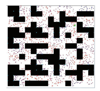
The initial state of particles distribution is shown in Fig. 4, in which the number of the particles is 2 000. The green arrow shows the robot's real position in the environment, the grey small circle indicates the initial position of the robot represented by the particle, and the black squares indicate the obstacles.
|
Fig.4 Initial state of particles distribution |
It can be seen from Fig. 4 that the particles at the initial time were distributed throughout the space.
The localization algorithm needs to predict the possible position of the robot based onits latest observations, and at the same time combines the real position of the robot at the next moment and performs a dynamic adjustment to trace the green arrow (Fig. 4). Comparing the simulation data of the IMCL algorithm with the AMCL, as shown in Fig. 5, the IMCL algorithm data was quickly recovered after localization loss.

|
Fig.5 Simulation data forAMCL and IMCL algorithms |
It can be seen from Fig. 5 that the error between the estimated value and the true value during the initial localization was big. With the running time, particles gathered near the real position of the robot and the error gradually decreased, while when the robot was "kidnapped", the error increased rapidly. The simulation data shows that the IMCL is superior to the AMCL in robot "kidnapping" detection, so it can be applied to solve the problem.
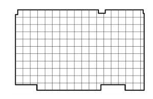
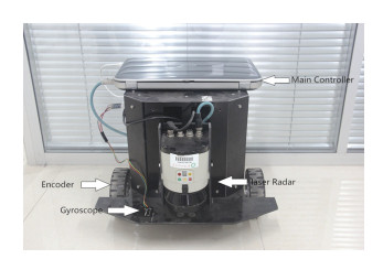
4.2 Experimental Analyses of LocalizationThispaper selects a laboratory of 10 500 mm×6 600 mm for the experimental scenario as shown in Fig. 6 and a robot localization experiment platform as shown in Fig. 7.
|
Fig.6 Robot localization test scenario |
|
Fig.7 Robot localization experiment platform |
The experimental analyses of different scenarios with different levels of complexity and different "kidnapping" situations were conducted to demonstrate the effectiveness of the proposed algorithm.
The mobile robot in this experiment mainly includes the following functional units.
Main control system: Based on Ubuntu 16.04 ROS operating system, the hardware supports 8 GB of DELL inspiration 5420 laptop.
Data acquisition sensor:The SICK lms111 laser radar is used as the environmental measurement sensor, which is in the 180-degree scanning range of the minimum angular resolution of 0.5 degrees and the maximum measurement distance of 20 m to meet the needs of indoor mobile robot localization.
Direction and displacement sensorsare encoder and FY-AHRS model gyroscope.
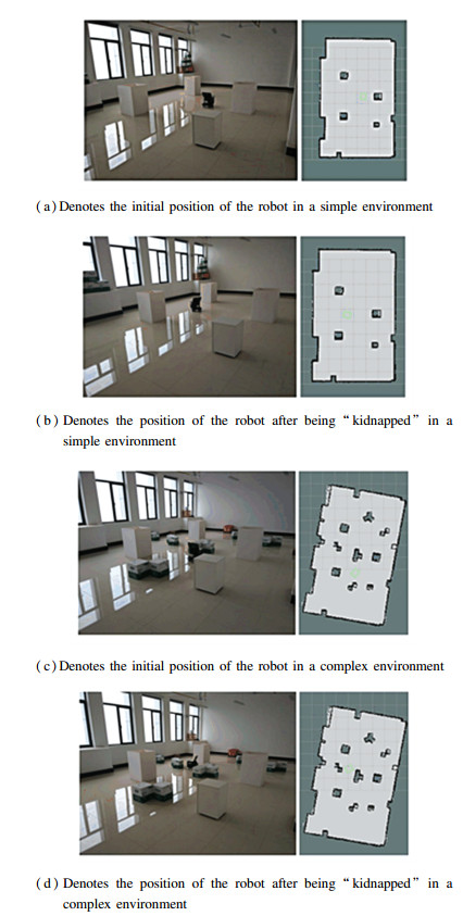
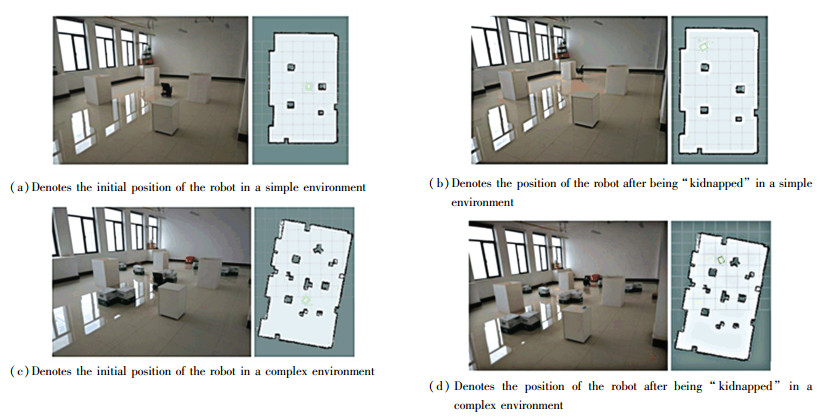
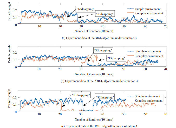
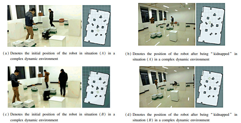
4.2.1 Analysis of the experimental data in different situations and environmentsThe experimental data was taken as the reference for the actual position of the robot and the position of the robot in the grid map during the experiment as shown in Fig. 8 and Fig. 9. The effectiveness of the IMCL algorithm was demonstrated by analyzing the changes in the weights of the particles during the experiment. The data provided in this paper were processed without affecting the true and valid data. The data analyses of the MCL, AMCL, and IMCL algorithms are shown in Fig. 10 and Fig. 11.
|
Fig.8 Scenarios for different algorithms under situation (A) |
|
Fig.9 Scenarios for different algorithms under situation (B) |
|
Fig.10 Comparison of relocalization results of different algorithms for situation (A) in different environments |

|
Fig.11 Comparison of relocalization results of different algorithms for situation (B) in different environments |
4.2.1.1 Data analysis under situation (A)
In situation (A), the robot was "kidnapped" near the real localization and it could observe the same road sign as before it was kidnapped.
The "kidnapping" data of the MCL, AMCL, and IMCL algorithms in situation (A) is shown in Fig. 10. The data of MCL and AMCL had consistency in simple and complex environments, which is also consistent with the variation of the weights of the particles in the standard MCL algorithm.
When the robot was in the situation of localization loss, the weights of the particles suddenly dropped, failed to recover in the MCL and AMCL localization algorithms, and fluctuated near a lower weight. However, from the data curve of the IMCL (Fig. 10), it can be seen that after a period of iterations, the weights returned to a stable state.
The experiments show that the improved robot had the ability to recover from situation (A) in both simple and complex environments.
4.2.1.2 Data analysis under situation (B)In situation (B), the robot was "kidnapped" far away from the real localization and it could not observe the same road sign as before it was "kidnapped".
Fig. 11 shows the experimental results of situation (B) in different environments. The data obtained under situation (B) had certain similar characteristics to that in situation (A). When the robot was in a state of localization loss, the weights of the particles would decrease, but as the number of iterations increased, only the weights of particles in the IMCL algorithm slowly rose back to a constant value, while that in the other two algorithms remained the same. Volatility around a lower value could not be recovered. Compared with situation (A), the recovery speed of IMCL algorithm in situation (B) was much slower. It is because there was a big change in the long-distance environmental characteristics, which led to a larger range of particle optimization.
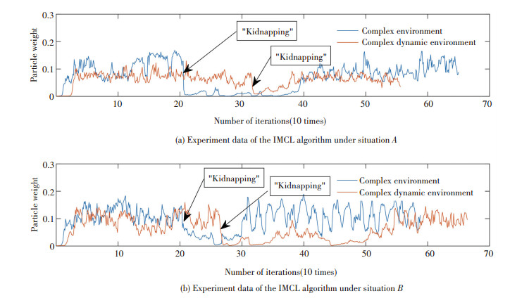
4.2.2 Data analysis of IMCLIn order to analyze the relocalization effect of the IMCL algorithm in a complex dynamic environment, further experiments were performed and the data is shown in Fig. 12.
|
Fig.12 IMCL algorithm for different situations in a complex dynamic environment |
Fig. 13 shows the experimental results of the IMCL algorithm in the complex dynamic environment. According to the localization data of the IMCL algorithm in complex and complex dynamic environments, the IMCL algorithm achieved self-recovery of localization loss for the two proposed situations in this work. From the results, it can be seen that the data obtained by the IMCL algorithm in different environments are basically consistent in terms of features. However, in the complex and complex dynamic environments, the characteristics of the weights of particles were obviously changed. Moreover, the average weight of ions varied greatly when the robot was in a "kidnapped" or a normal state, but this change was not the same in different environments. Overall, IMCL is proved robust on the issue of relocalization after "kidnapping".
|
Fig.13 Comparison of results obtained by IMCL algorithm under different situations in a complex dynamic environment |
Through the above three sets of experimental results, it can be concluded that the IMCL algorithm can solve the problem of robot's self-recovery from localization loss.
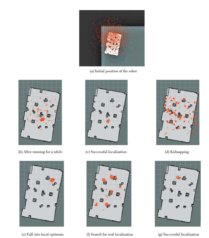
4.2.3 Analysis of situation (B) relocalization efficiency in different situationsFor situation (B), the IMCL had anisotropy in resolving the effectiveness of "kidnapping" relocalization. A more complex environment was selected for this experimental scenario. Fig. 14 demonstrates the seven images of the entire experimental process. The experiments in this paper mainly focus on the time needed for "kidnapping" iterations under different situations. Comparing situation (B1) with situation (B2) (Fig. 15), situation (B1) had an iterative average (less than 500) for 10 experiments which was significantly less than situation (B2) (greater than 500). During the experiment, it was found that robots achieved same localization loss and then recovered under different situations. Fig. 14(a) shows that the particles were in the initialized state. Figs. 14(b)-(c) show the robot's real position on the map by observing the model and sampling the motion model. Figs. 14(d)-(g) show the state of the robot being "kidnapped." The particles representing the robot in Figs. 14(d) and (f) began to determine the real position of the machine through the divergent sampling and the observation function weights. Fig. 14(e) shows that the particles were in a locally convergent state, but with the iteration of the motion model and observation model, they would re-diverge and finally converge to the real position of the robot.
|
Fig.14 Dynamic process of relocalization particles by localization loss of IMCL algorithm |

|
Fig.15 Comparison results of IMCL under different conditions in situation (B) |
As shown in Fig. 15, through multiple test results, the self-recovery of localization loss in situation (B1) was much faster. This experiment selected a complex environment and set relatively similar environments. When the robot was in a "kidnapping" state, by observing the particle dynamics, it can be found that the particles were clustered in a similar environment in situation (B2), which results in the proper positioning of the robot and more time for iteration. This makes it difficult for the iterations to increase, but over time, the iterations will increasingly approach the correct position and be accurately localized. The experiments also show that the complexity and similarity of the environments do affect the efficiency of robot localization.
A similar environment may cause the particles to fall into a local optimum, but the improved algorithm relocalization will work well that it guarantees that the robot will not fall into a local optimum during relocalization.
5 Summary and OutlookIn this paper, we propose an IMCL algorithm to solve the inability of robots to self-recover when their initial localization fails. Experiments conducted in simple and complex dynamic environments show that by improving the particle resampling function and the resampling mechanism, robots can relocate themselves from the "kidnapped" state to their real positions. Future studies can focus on extracting feature data from the indoor environment. A robot recognizable semantic map can be created, which can speed up the localization of the robot and the efficiency of relocalization after localization loss.
| [1] |
Liu H P, Zheng X M, Sun F C. Orientation estimate of indoor mobile robot using laser scans. Journal of Tsinghua University (Science and Technology), 2018, 58(7): 609-613. (  0) 0) |
| [2] |
Yu N, Wang S, Xu C. RGB-D based autonomous exploration and mapping of a mobile robot in unknown indoor environment. Robot, 2017, 39(6): 860-871. DOI:10.13973/j.cnki.robot.2017.0860 (  0) 0) |
| [3] |
Fox D, Burgard W, Thrun S. Markov localization for mobile robots in dynamic environments. AI Access Foundation, 1999, 11: 391-427. DOI:10.1613/jair.616 (  0) 0) |
| [4] |
Pfaff P, Burgard W, Fox D. Robust Monte-Carlo localization using adaptive likelihood models. In: Christensen H I. (eds) European Robotics Symposium 2006. Springer Tracts in Advanced Robotics. Berlin: Springer, 2006, 22: 181-194. DOI: 10.1007/11681120_15.
(  0) 0) |
| [5] |
Lee S, Lee S, Baek S. Erratum to: Vision-based kidnap recovery with SLAM for home cleaning robots. Journal of Intelligent & Robotic Systems, 2015, 78(1): 181. DOI:10.1007/s10846-014-0047-4 (  0) 0) |
| [6] |
Thrun S. Probabilistic Robotics. Communications of the ACM- Robots: Intelligence, Versatility, Adaptivity, 2002, 45(3): 52-57. DOI:10.1145/504729.504754 (  0) 0) |
| [7] |
Hess W, Kohler D, Rapp H, et al. Real-time loop closure in 2D LIDAR SLAM. IEEE International Conference on Robotics and Automation. Piscataway: IEEE, 2016.1271-1278. DOI: 10.1109/ICRA.2016.7487258.
(  0) 0) |
| [8] |
Oishi S, Jeong Y, Kurazume R, et al. ND voxel localization using large-scale 3D environmental map and RGB-D camera. 2013 IEEE International Conference on Robotics and Biomimetics. Piscataway: IEEE, 2013.538-545. DOI: 10.1109/ROBIO.2013.6739515.
(  0) 0) |
| [9] |
Mendoza R C, Bustamante P V, Medrano B, et al. 3D self-localization for humanoid robots using view regression and odometry. Proceedings of the 2015 12th International Conference on Electrical Engineering, Computing Science and Automatic Control. Piscataway: IEEE, 2015.1-5. DOI: 10.1109/ICEEE.2015.7357988.
(  0) 0) |
| [10] |
Yuen B L T, Sahari K S M, Rafaai Z F M. Improved map generation by addition of Gaussian noise for indoor SLAM using ROS. Journal of Robotics, Networking and Artificial Life, 2017, 4(2): 118-123. DOI:10.2991/jrnal.2017.4.2.3 (  0) 0) |
| [11] |
Park S Y, Lee G H. Mapping and localization of cooperative robots by ROS and SLAM in unknown working area. Proceedings of the 2017 56th Annual Conference of the Society of Instrument and Control Engineers of Japan(SICE). Piscataway: IEEE, 2017: 858-861.DOI: 10.23919/SICE.2017.8105741.
(  0) 0) |
| [12] |
Zhang Heng, Fan Xiaoping, Qi Zhihua. Research on adaptive Monte Carlo localization of mobile robot based on multiple hypothesis tracking. Acta Automatica Sinica, 2007, 33(9): 941-946. DOI:10.1360/aas-007-0941 (  0) 0) |
| [13] |
He F, Qin X L, Fang Y C. A genetic algorithm based autonomous localization strategy for mobile robots. Pattern Recognition and Artificial Intelligence, 2009, 22(1): 142-147. DOI:10.16451/j.cnki.issn1003-6059.2009.01.024 (  0) 0) |
| [14] |
Tian Y, Ma S. A double guarantee kidnapping detection in simultaneous localization and mapping. Proceedings of the 2014 International Conference on Multisensor Fusion and Information Integration for Intelligent Systems. Piscataway: IEEE, 2014.1-6. DOI: 10.1109/MFI.2014.6997744.
(  0) 0) |
| [15] |
Tian Y, Ma S. Probabilistic double guarantee kidnapping detection in SLAM. Robotics & Biomimetics, 2016, 3(1): 1-7. DOI:10.1186/s40638-016-0053-z (  0) 0) |
| [16] |
Tian Y, Ma S. Kidnapping detection and recognition in previous unknown environment. Journal of Sensors, 2017(120): 1-15. DOI:10.1155/2017/6468427 (  0) 0) |
| [17] |
Ying L U. Improved Monte Carlo Box localization algorithm for mobile nodes in Wireless Sensor Network. Computer Engineering & Applications, 2017, 53(10): 96-100. DOI:10.3778/j.issn.1002-8331.1512-0130 (  0) 0) |
| [18] |
Hanten R, Buck S, Otte S, et al. Vector-AMCL: Vector based adaptive Monte Carlo localization for indoor maps. Proceedings of the International Conference on Intelligent Autonomous Systems: Intelligent Autonomous Systems, 2016.403-416. DOI: 10.1007/978-3-319-48036-7_29.
(  0) 0) |
| [19] |
Fox D, Burgard W, Dellaert F, et al. Monte Carlo localization: Efficient position estimation for mobile robots. Proceedings of AAAI, 1999.343-349.
(  0) 0) |
 2020, Vol. 27


