Simultaneous Localization and Mapping (SLAM) is one of the key technologies in the autonomous navigation of robots[1-2]. As an important part of SLAM, loop closure detection is also concerned by many researchers, which can effectively solve the problem of position estimation drifting with time by judging whether the robot has arrived at the region that had been visited before, thus building a better global consistency map.
With the development of machine vision, it has become one of the most important technologies in the study of SLAM to use the information of environment acquired by vision sensors and image processing technology for place recognition and map construction.
At present, in the research of visual SLAM closed-loop detection method, cameras are used as sensors to obtain the environmental information of the scene, and the image matching method is employed to transform the visual closed-loop detection problem into sequential image matching problem. By computing the similarity between the current image and the historical image, the current image will be considered as the candidate loop for further processing when the similarity exceeds the threshold.
Currently, the algorithms about loop closure detection in visual SLAM are mainly based on point features. Cummins et al.[3] established a visual dictionary by using Scale-Invariant Feature Transform (SIFT) and Chow-Liu tree to build a scene appearance model in FAB-MAP. Galvez-López and Tardos[4] proposed DBoW and utilized FAST and BRIEF to extract key points and build binary descriptor which is used for k-means++ clustering to construct dictionary tree. Moreover, direct index and reverse index were used to speed up query and matching. In addition to point features, there are many other features, such as line feature, which can express structure information in environment and is more robust to changes of lighting, visual angle, and other environmental factors. Wang et al.[5] used the line segment extracted from ceiling images to compute the robot's motion, and the ceiling was utilized as the positive reference to determine the robot's global direction.Zhang et al.[6-7] constructed a closed-loop system based on line features and good results were obtained in both indoor and outdoor environments.
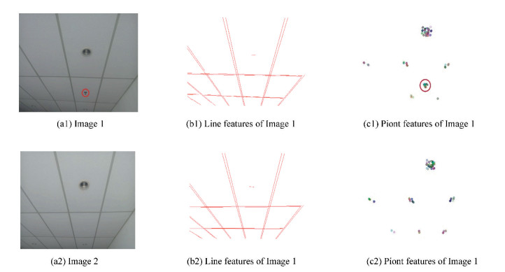
Point is a popular and widely used feature in visual SLAM. Point features perform well in strong texture scenes. However, when the scene lacks texture information or the blurred effect of the camera is caused by the rapid moving robot, the number of point features will be very small and inferior to line features in common man-made structured environment. Line features can reproduce structured scenes well, but its ability to represent texture information is weak. In high similar scenes like ceilings, line features are less capable of recognizing scenes. Furthermore, owing to the lack of point features, a group of meaningful visual words cannot be generated to describe images correctly, as shown in Fig. 1, but they can provide additional peculiarity to find correct matching in a database. Therefore, a loop closure detection algorithm based on point and line features is proposed in this paper to receive better performance in different environments.
|
Fig.1 Extract line and point features from two high similar ceiling images captured at different locations |
Here are the main contributions of this paper. Instead of building independent vocabulary trees for different feature types, a single vocabulary tree is constructed, which can combine different feature types and create mixed visual words to describe an image. In addition, different term frequency-inverted document frequency (TF-IDF) is computed for different type features. The approach based on hybrid feature can display texture and structured information of the scene at the same time, which also makes the closed-loop detection more robust in different environments.
2 Place RepresentationsOriented FAST and Rotated BRIEF (ORB) point feature descriptors and Line Band Descriptor (LBD) line feature descriptors are used in this paper, both of which are 256-bit descriptors, thus the construction of visual dictionary and the process of loop detection are simplified.
2.1 Point Feature Extraction and DescriptionThe technologies of point feature extraction, matching, and representation have become relatively mature in recent years. Point features are composed of two parts: key points and the descriptors. There are two kinds of description methods for point features: non-binary descriptor and binary descriptor. The most classical non-binary descriptor SIFT has strong robustness against illumination, scale, rotation, and other changes, but it has large computation cost and is poor in real-time. The speed of ORB extraction in the same image is two orders of magnitude faster than SIFT. ORB algorithm calculates the centroid C by using moment and determines the direction θ of FAST key points, which are corner-like points and are detected by comparing the gray intensity of some pixels in a Bresenham circle of radius 3. Through drawing a square patch Sb around each FAST key point and rotating the angle θ to obtain new point pairs in the neighborhood of feature points, the binary descriptor can be computed. For a key point p in an image, its corresponding BRIEF descriptor vector B(p) of length Lb is
| $ B^{i}(p)=\left\{\begin{array}{ll} 1, & \text { if } I\left(p+a_{i}\right) <I\left(p+b_{i}\right) \\ 0, & \text { otherwise } \ \ \forall i \in\left[1, L_{b}\right] \end{array}\right. $ | (1) |
where Bi(p) denotes the ith bit of the descriptor, I(·) is the intensity of the pixel in the smoothed image, and ai and bi are the 2-D offset of the randomly selected ith test point with respect to the center of the patch, with the value of
In this paper, line segments of the input image are extracted by Line Segment Detector (LSD)[8]. The input image was scaled to 80% of the original size by Gaussian subsampling, and the total number of pixels is 64% of the original size. Through subsampling, the aliasing and quantization artifacts in the image could be alleviated and even solved. Then a 2×2 mask was utilized to calculate the gradient of each pixel, and the gradient was macroscopically sorted using pseudo-sorting. Generally, regions with high gradient amplitude have strong edges, and pixel in the middle of edge usually has the highest gradient amplitude. When the gradient is less than the threshold, pixel will be discarded and will not be used to create line-support regions (LSR), which is generated by region growing algorithm. Unused points were used as seeds to check unused pixels in their neighborhood. If the difference between the level-line direction of a pixel and the LSR angle is within the tolerance T, the pixel can be included in the LSR until no pixel can be added to LSR. Lastly, count the number of aligned point in the rectangle and compute Number of False Alarms (NFA) to verify whether the LSR can be recognized as a line. LSD has the advantages of fast speed and it needs not to change the parameters.
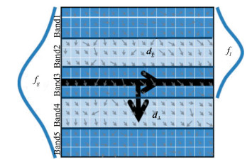
After extracting the key-line, LBD[9] was used to describe the line features. Compared with mean standard-deviation line descriptor (MSLD)[10], LBD has better matching effect and faster calculation speed. LBD is a non-binary line segment descriptor that can be transformed into binary descriptor easily. Similar to MSLD, LBD also sets up Band domain to compute descriptors and uses the concept of LSR. For a line segment, consider a rectangular region called LSR centered on it. As shown in Fig. 2, the region was divided into a set of bands parallel to the line segment, {B1, B2, B3, … Bm}, and the width of each band is w. Take the midpoint of the line segment as the origin and choose the line's direction dL and its clockwise vertical direction d⊥ to construct local 2-D coordinate system. Project all pixels in the LSR to this coordinate system as
| $ \boldsymbol{g}^{\prime}=\left(\boldsymbol{g}^{\mathrm{T}} \cdot d_{\perp}, \boldsymbol{g}^{\mathrm{T}} \cdot d_{L}\right) \triangleq\left(\boldsymbol{g}_{d_{\perp}, }^{\prime}, \boldsymbol{g}_{d_{L}}^{\prime}\right)^{\mathrm{T}} $ | (2) |
|
Fig.2 Diagram of LSR |
where g is the pixel gradient in the image coordinate system, and g' is the pixel gradient in the local coordinate system.
Then, global Gaussian function fg was applied to each row of LSR. For each band, a local Gaussian function fl was utilized to the rows of its nearest neighbor bands, which can reduce the effect of pixel gradient far from the line segment on Sdescriptors and reduce boundary effects. Based on gradients of adjacent band, each band Bj descriptor BDj can be computed. Connecting all the descriptors of the bands, the LBD descriptor can be obtained as follows:
| $ {\bf{LBD}} = {({\bf{B}}{{\bf{D}}^{\rm{T}}}_1, {\bf{B}}{{\bf{D}}^{\rm{T}}}_2, \ldots , {\bf{B}}{{\bf{D}}^{\rm{T}}}_m)^{\rm{T}}} $ | (3) |
The local gradients of each line in band Bj as well as their adjacent bands were summed separately, and the sum of each line was put together to form the following band description matrix BDMj:
| $ \mathbf{B D M}_{j}=\left(\begin{array}{cccc} v 1_{j}^{1} & v 1_{j}^{2} & \cdots & v 1_{j}^{n} \\ v 2_{j}^{1} & v 2_{j}^{2} & \cdots & v 2_{j}^{n} \\ v 3_{j}^{1} & v 3_{j}^{2} & \cdots & v 3_{j}^{n} \\ v 4_{j}^{1} & v 4_{j}^{2} & \cdots & v 4_{j}^{n} \end{array}\right) \in \mathbf{R}^{4 n} $ | (4) |
where
| $ \begin{aligned} v 1_{j}^{k} &=\gamma \sum\limits_{g^{\prime} d_{\perp}>0} g_{d_{\perp}}^{\prime}, v 2_{j}^{k}=\gamma \sum\limits_{g_{d_{\perp}}^{\prime}<0}-g_{d_{\perp}}^{\prime} \\ v 3_{j}^{k} &=\gamma \sum\limits_{g^{\prime}_{d_{l}}>0} g_{d_{l}}^{\prime}, v 4_{j}^{k}=\gamma \sum\limits_{g_{d_{l}}^{\prime}<0}-g_{d_{l}}^{\prime} \end{aligned} $ | (5) |
where γ=fg(k)fl(k) is the Gaussian coefficient,
| $ n = \left\{ \begin{array}{l} 2w, \;\;j = 1||m\\ 3w, \;\;{\rm{else}} \end{array} \right. $ |
Finally, construct BDj using the standard variance vector Sj and the mean vector Mj of the matrix BDMj as BDj =(MjT, SjT)∈R8, and bring them into
| $ {\bf{LBD}} = {(\mathit{\boldsymbol{M}}_1^{\rm{T}}, \mathit{\boldsymbol{S}}_1^{\rm{T}}, \mathit{\boldsymbol{M}}_2^{\rm{T}}, \mathit{\boldsymbol{S}}_2^{\rm{T}}, \ldots , \mathit{\boldsymbol{M}}_m^{\rm{T}}, \mathit{\boldsymbol{S}}_m^{\rm{T}})^{\rm{T}}} \in {{\bf{R}}^{8m}} $ | (6) |
In this paper, 32 pairs of vectors are extracted from LBD in a certain order, and an 8-bit binary string can be obtained by bitwise comparison. When the 32 binary strings were connected, a 256-dimensional binary vector was acquired. Similar to ORB descriptors, Hamming distance can be used to calculate the distance between LBD descriptors.
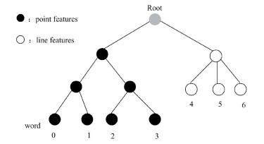
2.3 Visual DictionaryInspired by Ref. [11], this paper constructs a kind of visual dictionary which can integrate two different types of features, and establishes a database of mixed features. Since 32-dimensional ORB descriptors and LBD descriptors are very close in Euro-space, it is easy to cluster the two descriptors into a single visual word by mixing them together directly. Therefore, a label was set at the end of each descriptor to distinguish different feature types when describing the features. In the second layer of the dictionary tree, descriptors were classified by labels, and different types of descriptors were clustered by k-means++ method. The visual dictionary tree with hybrid line and point features is shown in Fig. 3.
|
Fig.3 Visual dictionary model with hybrid features |
The branch and depth of point features clustering are Kp=7, Lp=5, and the line feature clustering are Kl=6, Ll=5 in this paper. The degree of discrimination between different words was determined by TF-IDF to judge the weight of word i, which can be computed by
| $ {\omega _i} = {\rm{T}}{{\rm{F}}_i} \times {\rm{ID}}{{\rm{F}}_i} = \frac{{{n_i}}}{n} \times {\rm{log}}\frac{N}{{{N_i}}} $ | (7) |
Among them, ni is the number of word i in query image, n is the total number of words contained in the image, where different types of features correspond to different n, N is the sum total of images contained in the database, and Ni is the quantity of images containing the word i in the database.
The input image was divided into the nearest leaf node by calculating Hamming distance between the descriptor and the node in the visual dictionary. At last, the word vector corresponding to the image can be obtained as follows (w0 to wk is the word corresponding to the point features in the input image and wk+1 to wn is the word corresponding to the line feature):
| $ V = \{ \left( {{w_0}, {\omega _0}} \right), \left( {{w_1}, {\omega _1}} \right), \ldots \left( {{w_k}, {\omega _k}} \right), \ldots ({w_n}, {\omega _n})\} $ | (8) |
In order to make the result more reasonable and accurate, the similarity scores of different features of the image were calculated respectively and according to Ref. [11], certain weights were set to sum
| $ S = \mu S{\left( {{V_a}, {V_b}} \right)_p} + \left( {1 - \mu } \right)S{\left( {{V_a}, {V_b}} \right)_l} $ | (9) |
In Ref. [12], different types of features have the same importance (μ=0.5), but we think that it is necessary to adjust the parameter according to the environment. For example, for scenes with rich line features, the weight of line features is larger. Therefore, the value of μ was set as 0.15 for the case of few extractable point features, such as the ceiling image, 0.35 for the situation of general indoor environment, and 0.5 for the situation of abundant point features in campus outdoor environment. The value of μ is a weight approximately determined by experiments.
3.2 Loop Closure Candidate and Loop Closure ThresholdAfter calculating the similarity scores between images, time consistency checking and continuity checking were made to eliminate the mismatches, and finally the candidate loops were determined. Since images with similar time sequence will have similar scores when querying the database, the images with similar time sequence will be divided into a group as one match. The group with the highest score will be selected for the following continuity checking. If a suitable match is detected for consecutive frames before the current frame, which can be considered that there is a key frame, then the frame with the highest score in the current image matching group is selected as the candidate loop closure.
4 Experiment and AnalysisThis paper implements a loop closure detection algorithm in Windows10+VS2015. To extract and describe the point features and the line features, Opencv and related tools were utilized, noting that the descriptors are 32-dimension. Then, an improved visual dictionary with hybrid features based on DBOW3 was constructed. In the experiment of loop detection algorithm, the first 20 frames before the current frame were excluded to complete the time consistency detection. In the continuity detection, the frame image with the highest score in the group with the highest similarity score was chosen as the candidate loop closure. The value of μ was set as 0.35 in this experiment.
Fig. 4 shows the images query results in the database of different data dictionaries. In total, 440 images were collected by stereo camera from a building in the North China Electric Power University (NCEPU). The data on the left (220 images) were utilized to establish the database, and the data on the right (220 images) were used as the current input images. To verify the performance of the visual dictionary, the first 5 frames of image similarity were collected.

|
Fig.4 Query results from different visual dictionaries |
In Fig. 4, the scattered points on the upper left corner and the lower right corner are the result of the robot moving forward for a certain distance after a circle. It can be found that the query effect of the hybrid features dictionary was better than the single point and the line features. The number of scattered points in Fig. 4(a) and Fig. 4(b) was more than that in Fig. 4(c), and there were two faults (circle) in Fig. 4(a), indicating that the query failed.
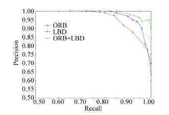
By setting different thresholds, the corresponding precision recall curves (PR curves) are drawn in Figs. 5-6. Fig. 5 shows the performace of three different methods in indoor dataset collected in the hall of a building in NCEPU, whereas Fig. 6 presents the performace of three different methods in CityCenter dataset which is an outdoor dataset.
|
Fig.5 PR curve of different algorithms in indoor dataset |
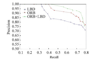
|
Fig.6 PR curve of different algorithms in outdoor dataset |
According to Fig. 5, the method based on point visual word was worse than line visual word, because the experimental scene contained abundant line features such as desk, chair, and bookcase, indicating that line feature had better discrimination than point feature.
In Fig. 6, the recall of the method based on single line feature was the smallest when the precision is 100%. Unlike indoor scenes, outdoor scenes did not have rich line features. Thus, the discrimination of line visual word was not as good as point visual word.
Hence, it can be concluded that the method with hybrid point-line feature was better than others. By fusing the two features, the algorithm was improved.
The execution time of each part of the algorithms shown in Fig. 5 is given in Table 1, in which the time of feature calculation and closed-loop detection in the closed-loop detection algorithm using the hybrid point-line feature was longer than that based on single features. The reason is that two features extraction of the image in the closed-loop detection will inevitably increase the corresponding computing time. Although the detection time was increased, the real-time requirements could still be fulfilled.
| Table 1 Average execution time with different closed-loop detection algorithms |
The proposed algorithm was compared with FAB-MAP in different datasets, and then the recall rates of the two algorithms were recorded when the precision is 100% (in Table 2).
| Table 2 Recall at 100% precision of two algorithms |
It can be seen in Table 2 that when the precision of loop detection is 100%, the recall rate of the proposed algorithm was significantly higher than those of FAB-MAP and IBuILD in three different environments, which confirms the feasibility and superiority of the proposed algorithm.
5 ConclusionsIn this paper, the proposed loop closure detection algorithm can reduce the common perceptual aliasing of BOW method, and can describe texture information as well as structure information. The similarity scores of different features between two images were calculated and summed in the proposed algorithm. Furthermore, by drawing the PR curves of three cases of single feature and hybrid features and comparing the proposed method with state-of-the-art methods in different datasets, it was found that the proposed method had better recall rates at 100% accuracy and it still satisfied the real-time requirement. Finally, experiments in different environments proved that the method based on hybrid feature had a better performance for various environments.
| [1] |
Thrun S, Leonard J J. Simultaneous Localization and Mapping. Siciliano B, Khatib O. Springer Handbook of Robotics. Berlin: Springer, 2008. 871-889. DOI: 10.1007/978-3-540-30301-5.
(  0) 0) |
| [2] |
Liu G, Hu Z. Fast loop closure detection based on holistic features from SURF and ORB. Robot, 2017, 39(1): 36-45. (in Chinese) DOI:10.13973/j.cnki.robot.2017.0036 (  0) 0) |
| [3] |
Cummins M, Newman P. FAB-MAP: Probabilistic localization and mapping in the space of appearance. International Journal of Robotics Research, 2008, 27(6): 647-665. DOI:10.1177/0278364908090961 (  0) 0) |
| [4] |
Galvez-López D, Tardos J D. Bags of binary words for fast place recognition in image sequences. IEEE Transactions on Robotics, 2012, 28(5): 1188-1197. DOI:10.1109/TRO.2012.2197158 (  0) 0) |
| [5] |
Wang H, Mou W, Suratno H, et al. Visual odometry using RGB-D camera on ceiling vision.Proceedings of IEEE International Conference on Robotics and Biomimetics. Piscataway: IEEE, 2013. 710-714. DOI: 10.1109/ROBIO.2012.6491051.
(  0) 0) |
| [6] |
Zhang G, Suh I H. Loop closure in a line-based SLAM. Journal of Korea Robotics Society, 2012, 7(2): 120-128. DOI:10.7746/jkros.2012.7.2.120 (  0) 0) |
| [7] |
Zhang G, Kang D H, Suh I H. Loop closure through vanishing points in a line-based monocular SLAM. Proceedings of 2012 IEEE International Conference on Robotics and Automation. Piscataway: IEEE, 2012. 4565-4570. DOI: 10.1109/ICRA.2012.6224759.
(  0) 0) |
| [8] |
Gioi R G V, Jakubowicz J, Morel J M, et al. LSD: A fast line segment detector with a false detection control. IEEE Transactions on Pattern Analysis and Machine Intelligence, 2010, 32(4): 722-732. DOI:10.1109/TPAMI.2008.300 (  0) 0) |
| [9] |
Zhang L, Koch R. An efficient and robust line segment matching approach based on LBD descriptor and pairwise geometric consistency. Journal of Visual Communication and Image Representation, 2013, 24(7): 794-805. DOI:10.1016/j.jvcir.2013.05.006 (  0) 0) |
| [10] |
Wang Z H, Wu F C, Hu Z Y. MSLD: A robust descriptor for line matching. Pattern Recognition, 2009, 42(5): 941-953. DOI:10.1016/j.patcog.2008.08.035 (  0) 0) |
| [11] |
Yang S, Mou W, Wang H, et al. Place recognition by combining multiple feature types with a modified vocabulary tree. Proceedings of 2015 International Conference on Image and Vision Computing New Zealand. Piscataway: IEEE, 2016. 1-6. DOI: 10.1109/IVCNZ.2015.7761547.
(  0) 0) |
| [12] |
Gomez-Ojeda R, Zuñiga-Noël D, Moreno F A, et al. PL-SLAM: A stereo SLAM system through the combination of points and line segments. IEEE Transactions on Robotics, 2019. 724-746.DOI: 10.1109/TRO.2019.2899783.
(  0) 0) |
| [13] |
Yin J, Li D, He G. Mobile robot loop closure detection using endpoint and line feature visual dictionary. Proceedings of 2017 2nd International Conference on Robotics and Automation Engineering. Piscataway: IEEE, 2018. 73-78. DOI: 10.1109/ICRAE.2017.8291356.
(  0) 0) |
| [14] |
Khan S, Wollherr D. IBuILD: Incremental bag of binary words for appearance based loop closure detection. Proceedings of 2015 IEEE International Conference on Robotics and Automation (ICRA). Piscataway: IEEE, 2015. 5441-5447. DOI: 10.1109/ICRA.2015.7139959.
(  0) 0) |
 2020, Vol. 27


