In the operation of public transportation system, it is vital to provide reliable and comfortable service for passengers. The key to solve the problem of bus operation and scheduling is to maintain the punctuality and stability of the service, so that passengers can effectively arrange their departure time and make informed decisions for travel choices. Meanwhile, when the normal operation is interfered, operators may take appropriate measures according to the real-time vehicle circumstances to adjust schedules and departure intervals (e.g., increase or reduce the speed, or prolong parking of some sites), so as to make the operation management more effective. This study on bus arrival time prediction method aims at improving the bus travel time prediction precision. Precisely predicted arrival time can help bus operators guarantee bus punctuality and reduce the passenger waiting time, thereby enhancing the bus attraction and competitiveness as well as promoting the intelligent transportation system (ITS) implementations.
Due to the stochastic property of traffic conditions and the subjectivity of drivers, it is difficult to accurately predict bus arrival time. Therefore, the modeling for bus arrival time prediction is not a straightforward task. However, the wide application of information technologies, such as radio frequency identification, smart card, and automatic vehicle location, has generated plenty of high-precision data and boosted bus arrival time prediction researches based on different kinds of data sources.
1.2 Literature ReviewVarious emerging and sophisticated algorithms have been designed and applied to solve the problem of bus arrival time prediction. According to Ma et al.[1], traffic prediction approaches have been transformed to intelligent computing from traditional statistical models. Compared with traditional models, the machine-learning technology is more competent in processing missing and extreme data, and needs little prior knowledge. Therefore, machine-learning approaches are often used to dispose multi-dimensional features with non-linear relationship, among which Artificial Neural Network (ANN) and Support Vector Machines (SVM) have achieved relatively good results for bus arrival time predictions.
1.2.1 ANNANN has become a popular tool in the domain of traffic prediction because of its flexible multi-layer structure, capability of handling high-dimensional data, and strong learning ability and generalization[1-2].Ji et al.[3] established the prediction model of bus arrival time based on wavelet neural network and used the particle swarm algorithm to optimize the model parameters.
1.2.2 SVMSVM transforms low-dimensional nonlinear problems into linear problems in a high-dimensional space problem by means of nonlinear transformation and solves high-dimensional problems by constructing kernel functions. SVM-based forecasting methods have been demonstrated with better performance than baseline in several studies[4-5].
A class of machine-learning techniques, named deep learning, is developing rapidly in recent years, which has been significantly improved in object detection, visual object recognition, speech recognition, and many other domains such as genomics and drug discovery[6]. The research on using deep learning techniques to predict bus arrival time directly is scant. However, the applications on other domains especially sequence task have considerable reference significance.
1.2.3 Recurrent neural networks (RNNs)/Long short-term memory (LSTM) networksRNNs have been verified to be adept at forecasting the next word in the sequence or the next character in the text[6-9]. As expounded in Ref. [6], in order to correct gradient explosion in RNNs, LSTM networks were proposed by adding special hidden units called forgotten gate and memory gate, whose natural behavior is to filter invalid ingredient and remember valid ingredient of inputs automatically for a long time. Ma et al.[1] established the LSTM network model to predict traffic speed based on coil data.
1.2.4 Convolutional neural networks (CNN)The powerful performance of CNN has been confirmed in many tasks where labelled samples are relatively sufficient. Zhang et al.[10] proposed a CNN-based model to predict the crowd flow in each region of a city, whose results demonstrated that the model improves accuracy significantly. Gebru et al.[11] used CNN and Google Street View to estimate the demographic makeup of the USA. Sainath et al.[12] proposed an architecture which combined the Conv with LSTM networks on a variety of large vocabulary tasks. Shi et al.[13] proposed the convolutional LSTM (ConvLSTM) for precipitation nowcasting, specifically predicting the future rainfall intensity over a relatively short period of time.
With the power of deep learning, we tried to apply this technology to bus arrival time predication in this paper. We were faced with and solved three main difficulties: a) which features are useful for bus arrival time prediction and how to extract these information from bus trajectory data; b) how to construct these features to conform to the input form of deep learning models and take advantage of the models; and c) how to adjust the model architecture to make it suitable for the problem of bus arrival time prediction.
The rest of this paper is organized as follows: Section 2 presents a formal description of the problem of bus arrival time prediction and an analysis of the temporal-spatial correlation between features and bus travel time prediction; Section 3 reveals the construction of the proposed model and the input; Section 4 provides a case study in Shenzhen bus system and analyzes the prediction performance of the proposed model compared with baseline models; and Section 5 gives the conclusion and discussion.
2 Formulation of Bus Arrival Time Prediction ProblemDefinition 1: Section s is the part of bus route between the s-th station and (s+1)-th station.
Definition 2: Shift i is the i-th running on bus route in one day.
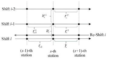
Based on the above definition, two features are described by brace in Fig. 1.
|
Fig.1 Symbols description in bus arrival time prediction problem |
(a) tsi is the bus travel time of shift i in section s.
| $ t_s^i = T_{s + 1}^i - T_s^i $ | (1) |
where Tsi and Ts+1i are bus arrival time of shift i at s-th and (s+1)-th stations, respectively.
(b) hsi is the headway of shift i at s-th station
| $ h_s^i = T_s^i - T_s^{i - 1} $ | (2) |
On the premise that the truth value Tsi has been obtained, the predict value of arrival time
| $ \hat T_{s + 1}^i = T_s^i + \hat t_s^i $ | (3) |
Thus, the problem of bus arrival time prediction at a target station can be transformed to the problem of bus travel time prediction in a target section.
Yu et al.[4] suggested that the travel time of the preceding bus that has just arrived at the station can be used to reflect the traffic conditions, and the headway can be used to reflect the timeliness of the bus travel times of the preceding buses.
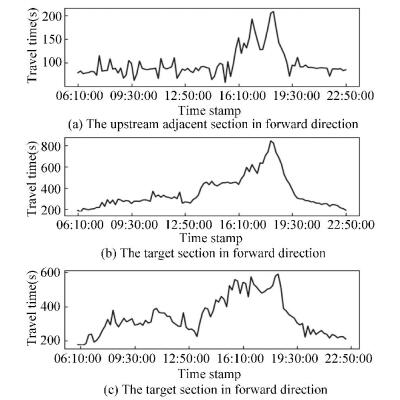
In our opinion, the headway and the travel time in a target section only utilize temporal information. It is easy to imagine that during evening peak periods, the bus travel time on the whole route including the target section will increase drastically. An actual observation is shown in Fig. 2. The change trend of the bus travel time in the target section had correlation with its adjacent sections and even with all other sections on the whole route.
|
Fig.2 Bus travel time in every five minutes during route operation hours |
Fig. 2 shows the common change tendency in a certain extent. At 7 a.m., the travel time began to rise and fluctuate. Until about 4 p.m., the travel time experienced a substantial increase and peaked at 6 p.m. After 7:30 p.m., the travel time returned to normal.
Thus, considering the spatial-temporal information, we extended to extract the two features from the whole route. Let ti be a set of bus travel time in continuous sections of route by shifts i.
| $ {t^i} = \{ t_s^i|s = 1,2, \cdots ,S - 1\} $ |
where S is the total number of stations on the route.
Likewise, let hi be a set of headway in continuous stations of route by shifts i.
| $ {h^i} = \{ h_s^i|s = 1,2, \cdots ,S - 1\} $ |
So far, all the information that has been discussed is confined to one direction of the route.
Definition 3: Re-Shift i is the last running in the opposite direction to shift i on the route, which has passed the target section before shift i, as shown in Fig. 1 by solid line with left arrows.
Although the direction is different, the majority traveling tracks of the Shift and Re-Shift are overlapping. The traffic condition of the section in reverse direction is similar to the forward direction in most time period, as shown in Fig. 2. Let tri and hri represent a set of bus travel time and headway by Re-Shift i, respectively.
Then, the problem of bus travel time prediction can be inducted as follows:
Problem 1: Given the historical observations {ti, hi|i=n-j, n-j+1, …, n} and {tri, hri|i=n-k, n-k+1, …, n}, predict tmn, where n is the target shift and m is the target section.
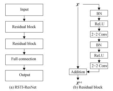
3 Residual Networks Based on Route Spatial-Temporal InformationFig. 3 shows the architecture of RSTI-ResNet, which is a framework modeling the route spatial-temporal information.
|
Fig.3 The overall scheme of the RSTI-ResNet and residual block |
3.1 Route Spatial-Temporal Information
A j×s matrix of bus travel time was constructed by historical observations {ti|i=n-j, n-j+1, …, n}, as shown in Fig. 4. The elements in a row of the matrix are the bus travel time of each section on route generated by a certain shift. The elements in a column of the matrix are the bus travel time of each shift passing a certain section. Likewise, a j×s matrix of bus travel time was constructed by historical observations {hi|i=n-j, n-j+1, …, n}. Then, we combined these two matrixes into a tensor Xf∈Rj×sf×2, as shown in Fig. 4, where R represents real number space, 1≤q≤m≤p≤S-1 and sr=p-q. If k < j, the missing element of Xf in the dimensionality of k is filled by 0.

|
Fig.4 Constitution of route temporal-spatial information |
The reverse direction information was constructed to a tensor Xr∈Rk×Sr×2 in the same way by the historical observations {tri, hri|i=n-k, n-k+1, …, n}.
Finally, a tensor X∈Rj×(sr+sf)×2 was achieved by concatenating Xr to Xf, corresponding to the top check in Fig. 3(a), as an input fed to the proposed model. The rows in tensor X represent the route spatial information while the columns denote the route temporal information.
Tentatively, a fraction of values in tensor X which had not been observed were taken place by the value 0. Take the bus travel time in downstream sections of the target section (i.e., {tsn|s≥m}) as an example. According to the precondition, the shift n has just arrived at station m when the bus travel time in section m would be predicted.
3.2 StructureThe structure of the proposed model framework consisting of two components, i.e., residual block and full connection, is inspired by the philosophy of Deep Residual Network proposed in Ref. [14].
3.2.1 Residual blockIn order to obtain the spatial correlation between the target section and other sections and the temporal correlation between the target shift and preceding shifts, it is necessary to design a multilayer CNN. A stack of convolutions can have further effects to capture the wide dependencies that exceed the size of their filters.
Residual learning was employed in the proposed model, which can gain accuracy from considerably increased depth. Residual learning has shown state-of-the-art results on multiple challenging recognition tasks, including object detection, image classification, localization, and segmentation[14]. Each residual block can be expressed in a general form[15] as follows:
| $ {x_{l + 1}} = h({x_l}) + F({x_l},{W_l}) $ | (4) |
where xl and xl+1 are input and output of the l-th block; h(xl)=xl is an identity mapping; Wl includes all learnable parameters in this unit; and F is the residual function, e.g., a stack of two 2×2 convolution layers with pre-activation: Batch Normalization[16] and ReLU[17], as shown in Fig. 3(b).
In the convolution layer, a filter handles the input Xlc from upper layer as
| $ X_l^{c + 1} = W_l^c*X_l^c $ | (5) |
where * denotes the convolutional operation and Xlc+1 is the output of the c-th convolution in the l-th unit.
3.2.2 Full connectionThe network ends with a 1-way fully-connected layer with linear. Ultimately, the output of full-connected layer is taken as the predict value of bus travel time.
Our RSTI-ResNet was trained to predict tmn by minimizing mean squared error between the true value and the predicted value with l2-regularizer as follows:
| $ L(\hat t_m^n;\theta ) = \left\| {t_m^n - \hat t_m^n} \right\|_2^2 + \lambda {\left\| \theta \right\|_2} $ | (6) |
where θ are all learnable parameters in the proposed model.
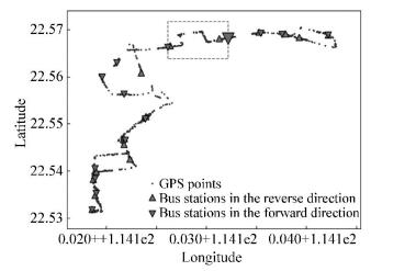
4 Experiments 4.1 DatasetThe trajectory data we used was taken from Shenzhen bus system, from Nov. 1st, 2015 to Apr. 30th, 2016. An all-day track of a bus running on route No. 10 is shown in Fig. 5, which presents the shape of the route. The biggest red triangle is the target station. The part of route enclosed by the dashed box is the target section.
|
Fig.5 An all-day track of a bus running on route No.10 |
From Fig. 5, it can be seen that the target section is the 10-th section in the forward direction and the 5-th section in the reverse direction. In our experiment, nine continue shifts including the target shift, the 8-th, 9-th, 10-th sections in the forward direction while night continue re-shifts, and the 5-th section in the reverse direction were selected to provide the route temporal-spatial information, meaning {sr, sf, j, k} is equal to {3, 1, 9, 9}. Thus, the size of inputs to RTSI-ResNet is 9×4×2.
4.2 Data PreprocessingExcept the actual bus arrival time at each station, our raw bus trajectory data recorded current time, speed, longitude, latitude, etc. A set of rules was provided to judge the bus arrival time from the raw bus trajectory data.
4.2.1 Scenario oneThere are one or more GPS points in the platform area, with which the value of the recorded bus speed is 0 km/h, as shown in Fig. 6(a). Then the current time recorded on the GPS point, which is the closest to the station coordinate, was selected as the actual bus arrival time.

|
Fig.6 Scenarios of GPS points located near the bus station |
4.2.2 Scenario two
There is no GPS point that satisfies the condition in Scenario one, and one or more GPS points are in inbound area and outbound area, as shown in Fig. 6(b). Then two GPS points which are the closest to station coordinate in inbound and outbound area are selected, e.g., GPS point 2 and GPS point 3 in Fig. 6(b).
The process of bus entering and leaving the station can be divided into three parts, as shown in Fig. 7, where VGP2(VGP3) and tGP2(tGP3) are the bus speed and current time recorded with GPS point 2(3).

|
Fig.7 Process of bus entering and leaving the station |
1) Part I: Inbound and deceleration. The bus at the GPS point 2 decelerates uniformly and runs ahead to an unknown position (Pos1). Va is the bus speed at Pos1.
2) Part II: Stop or pass station with a low speed. The bus keeps speed Va and runs to an unknown position (Pos2). The speed Va can be equal to 0 km/h if there are passengers getting on or off then the bus stops, or it is greater to 0 km/h if there is no passenger getting on or off then the bus passes platform with a low uniform speed. If Va=0 km/h, then Pos2 is Pos1 and S2=0 km.
3) Part III: Outbound and acceleration. The bus at Pos2 accelerates uniformly and runs ahead to the GPS point 3.
Then, a model was established to obtain the running time t1:
| $ {{\rm{min}}|{s_d} - ({s_1} + {s_2})} $ | (7) |
| $ {{t_1} + {t_2} + {t_3} = t} $ | (8) |
| $ {{s_1} + {s_2} + {s_3} = s} $ | (9) |
where ti and si are the bus running time and distance in part i, respectively. Formula (7) makes the Pos2 close to the station coordinate as much as possible. sd is the distance between GPS point 2 and station coordinate. Formula (8) constraints the duration in the process of entering and leaving station t=tGP3-tGP2. Formula (8) constraints the total running distance in the process. s is the distance between GPS point 2 and GPS point 3. The relational expressions among velocity, time, and distance are not introduced here. After solving the model, the arrival time is expressed as tGP2+t1.
4.2.3 Scenario threeThere are one or more GPS points only in either inbound or outbound area, as shown in Fig. 6(c). It is assumed that the process that the bus decelerates uniformly from Pos1 to station coordinate if Pos1 is in inbound area, or accelerates uniformly from station coordinate to Pos1 if Pos1 is in outbound area. The arrival time is tPos1 plus or subtract the running time.
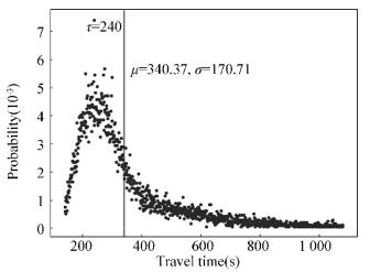
According to the above rules, the actual bus arrival time was obtained from the raw bus trajectory data. The distribution of bus travel time in the target section is shown in Fig. 8, where the vertical line indicates the mean value of the distribution; the mode τ, mean value μ, and standard deviation σ are equal to 240.00, 340.37, and 170.71, respectively. After data preprocessing, the features including bus travel time and headway that constitute the input of the model can be computed.
|
Fig.8 Distribution of bus travel time in target section |
4.3 Baselines
Our RSTL-ConvNet was compared with four baselines as follows.
4.3.1 ANN/SVMThe two features were fed only in the target section {tmi, hmi|i=n-8, …, n} to an artificial neural network with four fully-connected layers/support vector machine with kernel type of radial basis function.
4.3.2 RNN/LSTMRNN/LSTM is famous for time series prediction, which can capture the time dependent effectively. The RNN/LSTM model architecture is two RNN/LSTM layers followed by two fully-connected layers. The same features were fed to RNN/LSTM as ANN.
4.3.3 BiRNNBidirectional recurrent neural network (BiRNN) focuses on the context simultaneously, which accepts both the last moment output and next moment output of the hidden layers as input. The information about the next shifts (source of the next moment output) is unknown in our problem. The first several shifts which passed station m later than shift n in the same day of last week were regarded as the "next shifts" of shift n. The features {tmi, hmi, tmj, hmj·|i=n-8, …, n; j=n+1, .., n+4} were fed to a BiRNN model with two BiRNN layers and two fully-connected layers. tsj, hsj· are called historical future features.
4.3.4 FD-ConvNetThe ConvNet model, whose architecture is two convolution blocks followed by one fully-connected layer, is mainly inspired by VGG nets[18]. The convolution block is the combination of two convolution layers and one maxpooling layer. The same features were fed to FD-ConvNet as RSTI-ResNet but the reverse direction information was ignored.
4.4 HyperparametersIn ANN/RNN/LSTM/BiRNN model, except for the bottom layer, the upper layers have 512 hidden units in order to output one predicted value. The dropout probability in recurrent layers[19] and fully-connected layers[20] are 0.5. In FD-ConvNet, the previous convolution block uses 32 filters of size 2×2 and pooling strides 2, and the latter convolution block uses 64 filters of size 2×2 and pooling strides 2×1. In RSTI-ResNet model, the previous residual block uses 32 filters of size 2×2, and the latter residual block uses 64 filters of size 2×2 with downsampling of strides 2.
The batch size is 64. The model was trained using the asynchronous stochastic gradient descent (ASGD) optimization strategy. The learning rate is 0.001. Our data samples are about 15 000 where 80% are used for training and 20% are used for testing.
4.5 Evaluation MetricOur method was measured by Root Mean Square Error (RMSE) and Mean Absolute Percentage Error (MAPE) :
| $ {{\rm{RMSE}} = \sqrt {\frac{{\sum\nolimits_i {{{({y_i} - {{\hat y}_i})}^2}} }}{z}} } $ | (10) |
| $ {{\rm{MAPE}} = \frac{1}{z}\sum\nolimits_i {\frac{{|{y_i} - {{\hat y}_i}|}}{{{y_i}}}} } $ | (11) |
where y and
Table 1 shows the RMSE and MAPE for the seven methods.
| Table 1 Comparison among different methods |
It was found that the RSTI-ResNet was better than the baselines, and the accuracy of the proposed model improved effectively.
(a) RNN/LSTM/BiRNN had better performance than ANN/SVM, demonstrating the effectiveness of the RNN when handling temporal information. LSTM was superior to RNN in many time sequence tasks, but they were matched in the bus travel time prediction problem, at least on the features we fed, which may not embody the long-term dependent characteristics of LSTM.
(b) BiRNN did not perform better than RNN, indicating the futility of historical future features.
(c) FD-ResNet is a ResNet model, which only utilizes the forward direction information. It had an improvement compared with RNN, suggesting the contribution of spatial information to prediction. It is helpful to learn the increase or decrease tendency in nearby sections for bus travel time prediction in target section.
(d) RSTI-ResNet had a further improvement compared with the FD-ResNet, which demonstrates that the combination of the revere direction information and the forward direction information can reflect the road traffic conditions more comprehensively.
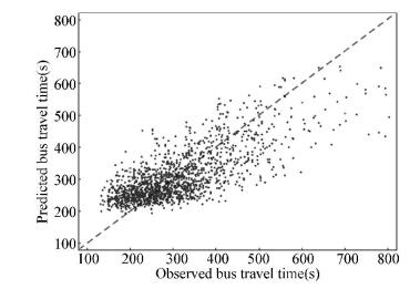
Fig. 9 shows the bus travel time predicted by the RSTI-ResNet against the true values in test set, where the black dash line is a guide line, on which the abscissa values are equal to the ordinate values.
|
Fig.9 Predictability of the proposed model |
4.7 Extension
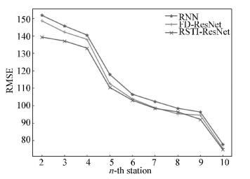
Then we relaxed the assumption. We tried to predict the bus arrival time at the target station Tm+1n when bus has arrived at stations m, m-1, m-2, …, 2, respectively. In our experiment, the target station was the 11-th station. Fig. 10 shows the RMSE for three methods. In general, the RTSI-ResNet was still better than others. Particularly, the advantage was more significant when the distance between bus and the target station was farther, which means less short-term information.
|
Fig.10 Predicted error in each previous station 5 Conclusions |
A point on a line represents the predicted error when buses are at the n-th station. For example, the far-left point on the green line shows that the RMSE of the predicted value of the bus arrival time the at 11-th station is 139.19 when buses are at the 2-nd station by the method of RTSI-ResNet.
A novel route spatial-temporal information based residual network for bus arrival time prediction was proposed. A set of rules were provided to judge the actual bus arrival time from the raw bus trajectory data. The proposed model was evaluated on the route No. 10 in Shenzhen bus systems, and the obtained results were better than other 7 baseline methods such as RNN/LSTM, ConvNet, and SVM, confirming that the model is more applicable to the bus travel time prediction problem. It demonstrates that using the spatial-temporal information of the whole route in both forward and reverse directions is effective on improving the prediction accuracy.
In our experiment, we tried to deepen the proposed model using four residual blocks and extracted features from 11 sections on the route No. 10, meaning the size of input was extended to 9×11×2. On one hand, the RMSE declined obviously under 45 s in validation set, and on the other, the RMSE raised beyond 100 s in the test set. The model was overfitting. It was considered that the number of our training samples (about 12000) was not large enough to cover the various complex scenarios in high dimensional characteristic. Bus arrival time prediction on a target route and any other routes are two different tasks because the data of any two routes may be in a different feature space while there is an obvious correlation between them. Considering the correlation, we will use the data of other bus routes to help train the model by transfer learning[21] in the future, which will enhance the performance of learning by avoiding the problem of train samples insufficient in target routes.
| [1] |
Ma X, Tao Z, Wang Y, et al. Long short-term memory neural network for traffic speed prediction using remote microwave sensor data. Transportation Research Part C: Emerging Technologies, 2015, 54: 187-197. DOI:10.1016/j.trc.2015.03.014 (  0) 0) |
| [2] |
Karlaftis M G, Vlahogianni E I. Statistical methods versus neural networks in transportation research: Differences, similarities and some insights. Transportation Research Part C: Emerging Technologies, 2011, 19(3): 387-399. DOI:10.1016/j.trc.2010.10.004 (  0) 0) |
| [3] |
Ji Y J, Lu J W, Chen X S, et al. Prediction model of bus arrival time based on particle swarm optimization and wavelet neural network. Journal of Transportation Systems Engineering and Information Technology, 2016, 16(3): 60-66. (in Chinese) (  0) 0) |
| [4] |
Yu B, Lam W H K, Tam M L. Bus arrival time prediction at bus stop with multiple routes. Transportation Research Part C: Emerging Technologies, 2011, 19(6): 1157-1170. DOI:10.1016/j.trc.2011.01.003 (  0) 0) |
| [5] |
Yu B, Ye T, Tian X M, et al. Bus travel-time prediction with a forgetting factor. Journal of Computing in Civil Engineering, 2012, 28(3): 06014002. DOI:10.1061/(ASCE)CP.1943-5487.0000274 (  0) 0) |
| [6] |
LeCun Y, Bengio Y, Hinton G. Deep learning. Nature, 2015, 521(7553): 436-444. DOI:10.1038/nature14539 (  0) 0) |
| [7] |
Wlodarczak P, Soar J, Ally M. Multimedia data mining using deep learning. Proceedings of 2015 Fifth International Conference on Digital Information Processing and Communications (ICDIPC). Piscataway: IEEE, 2015, 190-196. DOI:10.1109/ICDIPC.2015.7323027 (  0) 0) |
| [8] |
Sutskever I, Martens J, Hinton G. Generating Text with Recurrent Neural Networks. https://www.cs.utoronto.ca/~ilya/pubs/2011/LANG-RNN.pdf, 2019-04-12.
(  0) 0) |
| [9] |
Mikolov T, Sutskever I, Chen K, et al. Distributed Representations of Words and Phrases and Their Compositionality. https://papers.nips.cc/paper/5021-distributed-representations-of-words-and-phrases-and-their-compositionality.pdf, 2019-04-12.
(  0) 0) |
| [10] |
Zhang J, Zheng Y, Qi D. Deep Spatio-Temporal Residual Networks for Citywide Crowd Flows Prediction. https://www.aaai.org/ocs/index.php/AAAI/AAAI17/paper/viewFile/14501/13964, 2019-04-12.
(  0) 0) |
| [11] |
Gebru T, Krause J, Wang Y, et al. Using deep learning and Google Street View to estimate the demographic makeup of neighborhoods across the United States. Proceedings of the National Academy of Sciences, 2017, 114(50): 13108-13113. DOI:10.1073/pnas.1700035114 (  0) 0) |
| [12] |
Sainath T N, Vinyals O, Senior A, et al. Convolutional, long short-term memory, fully connected deep neural networks. Proceedings of 2015 IEEE International Conference on Acoustics, Speech and Signal Processing (ICASSP). Piscataway: IEEE, 2015, 4580-4584. DOI:10.1109/ICASSP.2015.7178838 (  0) 0) |
| [13] |
Shi X J, Chen Z, Wang H, et al. Convolutional LSTM Network: A Machine Learning Approach for Precipitation Nowcasting. http://de.arxiv.org/pdf/1506.04214, 2019-04-12.
(  0) 0) |
| [14] |
He K, Zhang X, Ren S, et al. Deep residual learning for image recognition. Proceedings of 2016 IEEE Conference on Computer Vision and Pattern Recognition (CVPR). Piscataway: IEEE, 2016, 770-778. DOI:10.1109/CVPR.2016.90 (  0) 0) |
| [15] |
He K, Zhang X, Ren S, et al. Identity Mappings in Deep Residual Networks. Leibe B, Matas J, Sebe N, et al. Computer Vision-ECCV 2016. Lecture Notes in Computer Science. Cham:Springer, 2016, 630-645. DOI:10.1007/978-3-319-46493-0_38 (  0) 0) |
| [16] |
Ioffe S, Szegedy C. Batch Normalization: Accelerating Deep Network Training by Reducing Internal Covariate Shift. https://arXiv preprint arXiv: 1502.03167, 2019-04-12.
(  0) 0) |
| [17] |
Krizhevsky A, Sutskever I, Hinton G E. ImageNet classification with deep convolutional neural networks. Advances in Neural Information Processing Systems, 2012, 25(2): 1097-1105. DOI:10.1145/3065386 (  0) 0) |
| [18] |
Simonyan K, Zisserman A. Very Deep Convolutional Networks for Large-Scale Image Recognition. http://arxiv.org/pdf/1409.1556.pdf, 2019-05-16.
(  0) 0) |
| [19] |
Zaremba W, Sutskever I, Vinyals O. Recurrent Neural Network Regularization. https://arXiv preprint arXiv:1409.2329, 2019-04-12.
(  0) 0) |
| [20] |
Srivastava N, Hinton G, Krizhevsky A, et al. Dropout: A simple way to prevent neural networks from overfitting. The Journal of Machine Learning Research, 2014, 15(1): 1929-1958. (  0) 0) |
| [21] |
Pan S J, Yang Q. A survey on transfer learning. IEEE Transactions on Knowledge and Data Engineering, 2010, 22(10): 1345-1359. DOI:10.1109/TKDE.2009.191 (  0) 0) |
 2020, Vol. 27


