2. Department of Automation, Nankai University, Tianjin 300071, China
Distributed coordination for multi-agent systems involves many aspects such as consensus and flocking. Consensus is a basic problem, in which the agent uses the distributed rule to make the system reach a common state. Gao et al.[1] studied the consensus with leader-following and without leader, respectively. Li et al.[2] demonstrated that all agents can achieve a consensus, even if the system have arbitrarily bounded communication delays.
In recent years, there are increasing studies on optimization problems. For instance, San et al.[3] presented a multi-objective optimization method to design the shape of membrane structures. Bi et al.[4] proposed a constrained optimization algorithm based on double populations to improve the distribution and convergence of the constrained optimization algorithms. However, previous researches focused on the distributed optimization problems and most of them are related to discrete-time algorithms[5-6]. Tsitsiklis et al.[7] originally presented a model for asynchronous distributed computation to achieve optimization. Li et al.[8] extended the optimization rule to the multi-agent systems, and directed topology played an important role in their research. Nedic et al.[9] formulated a projected rule for every agent in different convex sets to achieve optimization with a topology. At present, the distributed optimization problem has aroused interests of many scholars. By introducing a dynamic integrator, Wang et al.[10] presented a novel distributed rule for convex optimization. Based on the work in Ref. [10], other researchers[11-12] studied the optimization problem by strengthening conditions. Zhao et al.[13] formulated distribution optimization rule using the edge and adaptive design method on the basis of nodes. Studies in Refs. [14-15] achieved the finite-time consensus theoretically using the presented continuous forms of distributed non-smooth controllers. George and Subramanian[16]extended adaptive control with multiple models to the systems where the unknown parameters vary rapidly and frequently.
It is noteworthy that all the above results are related to the homogeneous multi-agents problems. The dynamics of the agents are always different due to the constraints in practical engineering applications, whereas the heterogeneous optimization problems have aroused little attention. Thus, given the actual situation, the study of distributed optimization with flocking of different dynamics systems is necessary both theoretically and practically. Zheng and Wang[17] created a sufficient condition of consensus for continuous-time heterogeneous systems without the measurements of velocity.
The innovations of this study are as follows. First, previous works primarily studied the consensus, while the distributed optimization problems of the heterogeneous systems have been rarely discussed. Accordingly, a distributed optimization algorithm was developed for heterogeneous system with flocking behavior to study how a group of agents can achieve optimization cooperatively. Second, this study proved the consensus and minimized the sum of the local cost functions for the heterogeneous systems.
Here is the structure of the paper. In Section 2, notations, concepts, and the preliminaries are presented, and a distributed control rule is proposed for heterogeneous multi-agent system with flocking behavior. The stability and the optimization are achieved in Section 3. The results are proved by a numerical case in Section 4, and the conclusions are drawn in Section 5.
2 Notations and Preliminaries 2.1 Algebraic Graph TheoryThe notations that will be used in this paper are presented in this part. AT denotes the transpose matrix of A, xT represents the transpose vector of x, and In ∈ Rn×n represents the unit matrix.
In general, an undirected graph G=(V, ε) is composed of a series of nodes V={1, 2, …, N} and a set of links ε. If i and j can be joined through a link (i, j), then (i, j)∈ε. Ni={j∈V:(j, i)∈ε} denotes the neighbor set of node i. If each pair of nodes in G has a link connected to each other, then the graph G is connected. A =[aij]∈ Rn×n is a weighted adjacent matrix of the graph G, which meets the conditions: 1)aii=0; 2)aij=aji>0, if (i, j)∈ε; and 3) aij=0, if (i, j)≠ε.
Let Λ =diag{d1, d2, …, dn}∈ Rn×n denote the degree matrix of the graph G, and
Consider the differential equation with a discontinuous right-hand side[19] as
| $ \dot y = f(y,t) $ | (1) |
where f: Rm× R→Rm is Lebesgue measurable and bounded. x(·) is called a Filippov solution to Eq. (1) on [t0, t1], if vector function x(·) meets the conditions in Ref. [20].
Lemma 1[21] Assume Ω1 is a compact set. Every Filippov solution to Eq. (1) beginning in Ω1 is unique and keeps in Ω1 for all t≥t0. Let V:Ω1→ R be regular function, which is independent of time with v≤0, ∀v∈
Assumption 1 The topology graph is undirected and connected.
Lemma 2[22] Considering a continuous differentiable convex function g(s): Rn→ R is minimized if and only if ∂g(s)=0.
Lemma 3[22] The second smallest eigenvalue λ2(L) of the Laplacian matrix L meets
| $ {\lambda _2}(\mathit{\boldsymbol{L}}) = {\rm{mi}}{{\rm{n}}_{{x^{\rm{T}}}{1_N} = ,x \ne 0}}\frac{{{\mathit{\boldsymbol{x}}^{\rm{T}}}\mathit{\boldsymbol{Lx}}}}{{{\mathit{\boldsymbol{x}}^{\rm{T}}}\mathit{\boldsymbol{x}}}} $ |
Definition 1[18] g(x) is σ-strongly(σ>0) convex if and only if
| $ (\mathit{\boldsymbol{x}} - \mathit{\boldsymbol{y}})(\nabla g(\mathit{\boldsymbol{x}}) - \nabla g(\mathit{\boldsymbol{y}})) \ge \mathit{\boldsymbol{\sigma }}{\left\| {\mathit{\boldsymbol{x}} - \mathit{\boldsymbol{y}}} \right\|^2} $ |
for σ>0, ∀x, y ∈Rn, and x≠y. If g(x) is σ-strongly convex and twice differentiable H(x) on x, then H(x) ≥σIn.
N(N>2) agent is considered with n-dimensional. For N agents, the number of the linear agents is m, labelled from 1 to m(m < N), and the rest are nonlinear agents. The dynamics of the system are respectively designed by
| $ \left\{ \begin{array}{l} {{\mathit{\boldsymbol{\dot x}}}_i}(t) = {\mathit{\boldsymbol{v}}_i}(t)\\ {{\mathit{\boldsymbol{\dot v}}}_i}(t) = f({\mathit{\boldsymbol{v}}_i}(t)) + {\mathit{\boldsymbol{u}}_i}(t),i = 1,2, \cdots ,m \end{array} \right. $ | (2) |
| $ \left\{ \begin{array}{l} {{\mathit{\boldsymbol{\dot x}}}_i}(t) = {\mathit{\boldsymbol{v}}_i}(t)\\ {{\mathit{\boldsymbol{\dot v}}}_i}(t) = {\mathit{\boldsymbol{u}}_i}(t),i = m + 1,m + 2, \cdots ,N \end{array} \right. $ | (3) |
where xi(t) ∈ Rn is the position of the agent i, vi(t)∈ Rn represents the velocity of the agent i, ui(t) is the control law of the agent i, and f(vi) is non-linear continuous function.
Assumption 2 There exists a constant 0 < ω≤1, for i=1, 2, …, m, such that ‖f(vi)‖≤ω ‖ vi‖.
The purpose of this paper is to devise a controller for Eqs. (2) and (3) that enables all agents to achieve optimization using local interactive information.
| $ {\rm{min}}\sum\limits_{i = 1}^N {{g_i}} (\mathit{\boldsymbol{s}}),\mathit{\boldsymbol{s}} \in {{\bf{R}}^n} $ | (4) |
where gi(s) :Rn →R is a local cost function known only to agent i, and gi(s) meets Assumptions 3 and 4.
Assumption 3 The local cost function gi(s):Rn →R is convex, differentiable, and meets
| $ {g_i}(\mathit{\boldsymbol{s}}) = {\mathit{\boldsymbol{s}}^{\rm{T}}}{\mathit{\boldsymbol{A}}_i}\mathit{\boldsymbol{s}} $ | (5) |
where
The above problem is transformed into the minimization problem of function as follows:
| $ \mathop {{\rm{min}}}\limits_{\mathit{\boldsymbol{v}} \in {{\bf{R}}^n}} \sum\limits_{i = 1}^N {{g_i}} ({\mathit{\boldsymbol{v}}_i}){\kern 1pt} {\kern 1pt} {\kern 1pt} {\rm{s}}{\rm{.t}}{\rm{.}}{\kern 1pt} {\kern 1pt} {\kern 1pt} {\mathit{\boldsymbol{v}}_i} = {\mathit{\boldsymbol{v}}_j} $ | (6) |
Assumption 4 Each function gi(vi) has a non-empty optimal solution set. Namely, there exists vi*∈ Rn which satisfies that gi(vi*) is minimum.
3 Main ResultsA distributed rule is presented, which makes the velocities of the agents the same and minimizes the function gi(vi).
| $ {\mathit{\boldsymbol{u}}_i} = - \sum\limits_{j = 1}^N {{a_{ij}}} ({\mathit{\boldsymbol{v}}_i} - {\mathit{\boldsymbol{v}}_j}) - \sum\limits_{j = 1}^N {{a_{ij}}} {\rm{sgn}} ({\mathit{\boldsymbol{v}}_i} - {\mathit{\boldsymbol{v}}_j}) + {\varphi _i} $ | (7) |
where
| $ {\varphi _i} = - H_i^{ - 1}({\mathit{\boldsymbol{v}}_i})\left( {\nabla {g_i}({\mathit{\boldsymbol{v}}_i}) + \frac{{\partial \nabla {g_i}({\mathit{\boldsymbol{v}}_i})}}{{\partial t}}} \right) $ |
aij describes the communication weight between agents i and j, and sgn(·) represents the signum function. It is noteworthy that φi relies merely on the velocity of the agent i. The twice differentiable function of the function gi(vi) with respect to vi is Hessian Hi(vi). Since the control rule developed in this paper contains sign functions, the system (2)-(3) has Filippov solution[19].
Theorem 1 For the multi-agent system (2)-(3) with the controller (7), all agents asymptotically reach a consensus if λ2(L) ≥σ-1λ*+ω.
Proof As can be seen from Eqs. (2)-(3), the closed-loop is
| $ \begin{array}{l} {{\mathit{\boldsymbol{\dot v}}}_i} = - \sum\limits_{i = 1}^N {{a_{ij}}} ({\mathit{\boldsymbol{v}}_i} - {\mathit{\boldsymbol{v}}_j}) - \sum\limits_{i = 1}^N {{a_{ij}}} {\rm{sgn}} ({\mathit{\boldsymbol{v}}_i} - {\mathit{\boldsymbol{v}}_j}) + \\ {\kern 1pt} {\kern 1pt} {\kern 1pt} {\kern 1pt} {\kern 1pt} {\kern 1pt} {\kern 1pt} {\kern 1pt} {\kern 1pt} {\kern 1pt} {\kern 1pt} {\kern 1pt} {\kern 1pt} {\kern 1pt} {\kern 1pt} {\kern 1pt} {\kern 1pt} {\kern 1pt} {\kern 1pt} {\kern 1pt} {\kern 1pt} {\kern 1pt} {\kern 1pt} {\kern 1pt} {\kern 1pt} {\varphi _i} + f({\mathit{\boldsymbol{v}}_i}) \end{array} $ | (8) |
Clearly, the right-hand side of Eq. (8) is discontinuous. Therefore, differential inclusions and non-smooth analysis can be used to illustrate the stability of system (2)-(3)[20] as
| $ \begin{array}{l} {{\mathit{\boldsymbol{\dot v}}}_i}{ \in ^{{\rm{a}}{\rm{.e}}{\rm{.}}}}\kappa [ - \sum\limits_{i = 1}^N {{a_{ij}}} ({\mathit{\boldsymbol{v}}_i} - {\mathit{\boldsymbol{v}}_j}) - \sum\limits_{i = 1}^N {{a_{ij}}} {\rm{sgn}} ({\mathit{\boldsymbol{v}}_i} - {\mathit{\boldsymbol{v}}_j}) + \\ {\kern 1pt} {\kern 1pt} {\kern 1pt} {\kern 1pt} {\kern 1pt} {\kern 1pt} {\kern 1pt} {\kern 1pt} {\kern 1pt} {\kern 1pt} {\kern 1pt} {\kern 1pt} {\kern 1pt} {\kern 1pt} {\kern 1pt} {\kern 1pt} {\kern 1pt} {\kern 1pt} {\kern 1pt} {\kern 1pt} {\kern 1pt} {\kern 1pt} {\varphi _i} + f({\mathit{\boldsymbol{v}}_i})] \end{array} $ |
where a.e. means "almost everywhere". Define the following function as
| $ {\mathit{\boldsymbol{V}}_1} = \frac{1}{2}\sum\limits_{i = 1}^N {\mathit{\boldsymbol{v}}_i^{\rm{T}}} {\mathit{\boldsymbol{v}}_i} $ |
From the properties of κ in Ref. [21], the set-valued Lie derivative of V(t) with on time along Eq.(8) is described as
| $ \begin{array}{l} {{\mathit{\boldsymbol{\dot {\tilde V}}}}_1} \in \kappa [\sum\limits_{i = 1}^N {\mathit{\boldsymbol{v}}_i^{\rm{T}}} {\mathit{\boldsymbol{u}}_i} + \sum\limits_{i = 1}^m {\mathit{\boldsymbol{v}}_i^{\rm{T}}} f({\mathit{\boldsymbol{v}}_i})] \in \\ \begin{array}{*{20}{l}} {{\kern 1pt} {\kern 1pt} {\kern 1pt} {\kern 1pt} {\kern 1pt} {\kern 1pt} {\kern 1pt} {\kern 1pt} {\kern 1pt} {\kern 1pt} {\kern 1pt} {\kern 1pt} {\kern 1pt} {\kern 1pt} {\kern 1pt} {\kern 1pt} {\kern 1pt} {\kern 1pt} {\kern 1pt} {\kern 1pt} {\kern 1pt} {\kern 1pt} {\kern 1pt} {\kern 1pt} {\kern 1pt} {\kern 1pt} {\kern 1pt} \kappa [ - \sum\limits_{i = 1}^N {\sum\limits_{j = 1}^N {{a_{ij}}} } \mathit{\boldsymbol{\nu }}_i^{\rm{T}}({\mathit{\boldsymbol{v}}_i} - {\mathit{\boldsymbol{v}}_j}) - }\\ {{\kern 1pt} {\kern 1pt} {\kern 1pt} {\kern 1pt} {\kern 1pt} {\kern 1pt} {\kern 1pt} {\kern 1pt} {\kern 1pt} {\kern 1pt} {\kern 1pt} {\kern 1pt} {\kern 1pt} {\kern 1pt} {\kern 1pt} {\kern 1pt} {\kern 1pt} {\kern 1pt} {\kern 1pt} {\kern 1pt} {\kern 1pt} {\kern 1pt} {\kern 1pt} {\kern 1pt} {\kern 1pt} {\kern 1pt} \sum\limits_{i = 1}^N {\sum\limits_{j = 1}^N {{a_{ij}}} } \mathit{\boldsymbol{v}}_i^{\rm{T}} {\rm{sgn}} ({\mathit{\boldsymbol{v}}_i} - {\mathit{\boldsymbol{v}}_j}) + } \end{array}\\ \begin{array}{*{20}{l}} {{\kern 1pt} {\kern 1pt} {\kern 1pt} {\kern 1pt} {\kern 1pt} {\kern 1pt} {\kern 1pt} {\kern 1pt} {\kern 1pt} {\kern 1pt} {\kern 1pt} {\kern 1pt} {\kern 1pt} {\kern 1pt} {\kern 1pt} {\kern 1pt} {\kern 1pt} {\kern 1pt} {\kern 1pt} {\kern 1pt} {\kern 1pt} {\kern 1pt} {\kern 1pt} {\kern 1pt} {\kern 1pt} {\kern 1pt} \sum\limits_{i = 1}^N {\mathit{\boldsymbol{v}}_i^{\rm{T}}} {\varphi _i} + \sum\limits_{i = 1}^m {\mathit{\boldsymbol{v}}_i^{\rm{T}}} f({\mathit{\boldsymbol{v}}_i})] \in }\\ {{\kern 1pt} {\kern 1pt} {\kern 1pt} {\kern 1pt} {\kern 1pt} {\kern 1pt} {\kern 1pt} {\kern 1pt} {\kern 1pt} {\kern 1pt} {\kern 1pt} {\kern 1pt} {\kern 1pt} {\kern 1pt} {\kern 1pt} {\kern 1pt} {\kern 1pt} {\kern 1pt} {\kern 1pt} {\kern 1pt} {\kern 1pt} {\kern 1pt} {\kern 1pt} {\kern 1pt} {\kern 1pt} {\kern 1pt} \kappa [ - \sum\limits_{i = 1}^N {\sum\limits_{j = 1}^N {{a_{ij}}} } \mathit{\boldsymbol{v}}_i^{\rm{T}}({\mathit{\boldsymbol{v}}_i} - {\mathit{\boldsymbol{v}}_j}) - } \end{array}\\ \begin{array}{*{20}{l}} {{\kern 1pt} {\kern 1pt} {\kern 1pt} {\kern 1pt} {\kern 1pt} {\kern 1pt} {\kern 1pt} {\kern 1pt} {\kern 1pt} {\kern 1pt} {\kern 1pt} {\kern 1pt} {\kern 1pt} {\kern 1pt} {\kern 1pt} {\kern 1pt} {\kern 1pt} {\kern 1pt} {\kern 1pt} {\kern 1pt} {\kern 1pt} {\kern 1pt} {\kern 1pt} {\kern 1pt} {\kern 1pt} {\kern 1pt} \frac{1}{2}\sum\limits_{i = 1}^N {\sum\limits_{j = 1}^N {{a_{ij}}} } ({\mathit{\boldsymbol{v}}_i} - {\mathit{\boldsymbol{v}}_j}) {\rm{sgn}} ({\mathit{\boldsymbol{v}}_i} - {\mathit{\boldsymbol{v}}_j}) + }\\ {{\kern 1pt} {\kern 1pt} {\kern 1pt} {\kern 1pt} {\kern 1pt} {\kern 1pt} {\kern 1pt} {\kern 1pt} {\kern 1pt} {\kern 1pt} {\kern 1pt} {\kern 1pt} {\kern 1pt} {\kern 1pt} {\kern 1pt} {\kern 1pt} {\kern 1pt} {\kern 1pt} {\kern 1pt} {\kern 1pt} {\kern 1pt} {\kern 1pt} {\kern 1pt} {\kern 1pt} {\kern 1pt} {\kern 1pt} \sum\limits_{i = 1}^N {\mathit{\boldsymbol{v}}_i^{\rm{T}}} {\varphi _i} + \sum\limits_{i = 1}^m {\mathit{\boldsymbol{v}}_i^{\rm{T}}} f({\mathit{\boldsymbol{v}}_i})]} \end{array} \end{array} $ |
By using ‖f(vi)‖≤ω ‖vi‖, one gets
| $ \begin{array}{*{20}{l}} {\mathit{\boldsymbol{\dot {\tilde V}}} \le - \sum\limits_{i = 1}^N {\sum\limits_{j = 1}^N {{a_{ij}}} } \mathit{\boldsymbol{v}}_i^{\rm{T}}({\mathit{\boldsymbol{v}}_i} - {\mathit{\boldsymbol{v}}_j}) - }\\ {{\kern 1pt} {\kern 1pt} {\kern 1pt} \frac{1}{2}\sum\limits_{i = 1}^N {\sum\limits_{j = 1}^N {{a_{ij}}} } {{({\mathit{\boldsymbol{v}}_i} - {\mathit{\boldsymbol{v}}_j})}^{\rm{T}}} {\rm{sgn}} ({\mathit{\boldsymbol{v}}_i} - {\mathit{\boldsymbol{v}}_j}) + }\\ {{\kern 1pt} {\kern 1pt} {\kern 1pt} |\sum\limits_{i = 1}^N {\mathit{\boldsymbol{v}}_i^{\rm{T}}} {\varphi _i}| + \sum\limits_{i = 1}^m \omega {{\left\| {{\mathit{\boldsymbol{v}}_i}} \right\|}^2}} \end{array} $ |
Let V=[ v1T, v2T, …, vNT]T, we have
| $ \begin{array}{l} \begin{array}{*{20}{l}} {-\sum\limits_{i = 1}^N {\sum\limits_{j = 1}^N {{a_{ij}}} } \mathit{\boldsymbol{v}}_i^{\rm{T}}({\mathit{\boldsymbol{v}}_i} - {\mathit{\boldsymbol{v}}_j}) - \frac{1}{2}\sum\limits_{i = 1}^N {\sum\limits_{j = 1}^N {{a_{ij}}} } {{({\mathit{\boldsymbol{v}}_i} - {\mathit{\boldsymbol{v}}_j})}^{\rm{T}}} \times }\\ { {\rm{sgn}} ({\mathit{\boldsymbol{v}}_i} - {\mathit{\boldsymbol{v}}_j}) = - {\mathit{\boldsymbol{V}}^{\rm{T}}}(\mathit{\boldsymbol{L}} \otimes {\mathit{\boldsymbol{I}}_n})\mathit{\boldsymbol{V}} - \frac{1}{2}{{\left\| {{\mathit{\boldsymbol{D}}^{\rm{T}}} \otimes {\mathit{\boldsymbol{I}}_n}\mathit{\boldsymbol{V}}} \right\|}_1}} \end{array}\\ |\sum\limits_{i = 1}^N {\mathit{\boldsymbol{v}}_i^{\rm{T}}} {\varphi _i}| = |\sum\limits_{i = 1}^N {\mathit{\boldsymbol{v}}_i^{\rm{T}}} ( - H_i^{ - 1}({\mathit{\boldsymbol{v}}_i})\nabla {g_i}({\mathit{\boldsymbol{v}}_i}))| = \\ \begin{array}{*{20}{l}} {|\sum\limits_{i = 1}^N {\mathit{\boldsymbol{v}}_i^{\rm{T}}} (\mathit{\boldsymbol{H}}_i^{ - 1}({\mathit{\boldsymbol{v}}_i})\nabla {g_i}({\mathit{\boldsymbol{v}}_i}))| \le }\\ {|\sum\limits_{i = 1}^N {\mathit{\boldsymbol{v}}_i^{\rm{T}}} ({\sigma ^{ - 1}}{\mathit{\boldsymbol{A}}_i}{\mathit{\boldsymbol{v}}_i})| \le |\sum\limits_{i = 1}^N {\sum\limits_{j = 1}^N {\mathit{\boldsymbol{v}}_i^{\rm{T}}} } ({\sigma ^{ - 1}}{\mathit{\boldsymbol{A}}_i}{\mathit{\boldsymbol{v}}_i})| = }\\ {{\sigma ^{ - 1}}{\mathit{\boldsymbol{V}}^{\rm{T}}}\mathit{\boldsymbol{BV}}}\\ {{\kern 1pt} {\kern 1pt} {\kern 1pt} {\kern 1pt} \sum\limits_{i = 1}^m \mathit{\boldsymbol{\omega }} {{\left\| {{\mathit{\boldsymbol{v}}_i}} \right\|}^2} \le \sum\limits_{i = 1}^N \mathit{\boldsymbol{\omega }} {{\left\| {{\mathit{\boldsymbol{v}}_i}} \right\|}^2} = \mathit{\boldsymbol{\omega }}{\mathit{\boldsymbol{V}}^{\rm{T}}}\mathit{\boldsymbol{V}}} \end{array} \end{array} $ |
Then, it yields
| $ \begin{array}{l} \mathit{\boldsymbol{\dot {\tilde V}}} \le - {\mathit{\boldsymbol{V}}^{\rm{T}}}(\mathit{\boldsymbol{L}} \otimes {\mathit{\boldsymbol{I}}_n})\mathit{\boldsymbol{V}} - \frac{1}{2}{\left\| {{\mathit{\boldsymbol{D}}^{\rm{T}}} \otimes {\mathit{\boldsymbol{I}}_n}\mathit{\boldsymbol{V}}} \right\|_1} + \\ {\kern 1pt} {\kern 1pt} {\kern 1pt} {\kern 1pt} {\kern 1pt} {\kern 1pt} {\kern 1pt} {\kern 1pt} {\kern 1pt} {\kern 1pt} {\kern 1pt} {\kern 1pt} {\kern 1pt} {\kern 1pt} {\kern 1pt} {\kern 1pt} {\kern 1pt} {\kern 1pt} {\kern 1pt} {\kern 1pt} {\kern 1pt} {\kern 1pt} {\kern 1pt} {\kern 1pt} {\kern 1pt} {\kern 1pt} {\sigma ^{ - 1}}{\mathit{\boldsymbol{V}}^{\rm{T}}}\mathit{\boldsymbol{BV}} + \mathit{\boldsymbol{\omega }}{\mathit{\boldsymbol{V}}^{\rm{T}}}\mathit{\boldsymbol{V}} \le \\ \begin{array}{*{20}{l}} {{\kern 1pt} {\kern 1pt} {\kern 1pt} {\kern 1pt} {\kern 1pt} {\kern 1pt} {\kern 1pt} {\kern 1pt} {\kern 1pt} {\kern 1pt} {\kern 1pt} {\kern 1pt} {\kern 1pt} {\kern 1pt} {\kern 1pt} {\kern 1pt} {\kern 1pt} {\kern 1pt} {\kern 1pt} {\kern 1pt} {\kern 1pt} {\kern 1pt} {\kern 1pt} {\kern 1pt} {\kern 1pt} - {\mathit{\boldsymbol{V}}^{\rm{T}}}(\mathit{\boldsymbol{L}} \otimes {\mathit{\boldsymbol{I}}_n})\mathit{\boldsymbol{V}} - \frac{1}{2}\sqrt {\mathit{\boldsymbol{L}} \otimes {\mathit{\boldsymbol{I}}_n}} \left\| \mathit{\boldsymbol{V}} \right\| + }\\ {{\kern 1pt} {\kern 1pt} {\kern 1pt} {\kern 1pt} {\kern 1pt} {\kern 1pt} {\kern 1pt} {\kern 1pt} {\kern 1pt} {\kern 1pt} {\kern 1pt} {\kern 1pt} {\kern 1pt} {\kern 1pt} {\kern 1pt} {\kern 1pt} {\kern 1pt} {\kern 1pt} {\kern 1pt} {\kern 1pt} {\kern 1pt} {\kern 1pt} {\kern 1pt} {\kern 1pt} {\kern 1pt} {\sigma ^{ - 1}}{\mathit{\boldsymbol{V}}^{\rm{T}}}\mathit{\boldsymbol{BV}} + \mathit{\boldsymbol{\omega }}{\mathit{\boldsymbol{V}}^{\rm{T}}}\mathit{\boldsymbol{V}} = } \end{array}\\ \begin{array}{*{20}{l}} {{\kern 1pt} {\kern 1pt} {\kern 1pt} {\kern 1pt} {\kern 1pt} {\kern 1pt} {\kern 1pt} {\kern 1pt} {\kern 1pt} {\kern 1pt} {\kern 1pt} {\kern 1pt} {\kern 1pt} {\kern 1pt} {\kern 1pt} {\kern 1pt} {\kern 1pt} {\kern 1pt} {\kern 1pt} {\kern 1pt} {\kern 1pt} {\kern 1pt} {\kern 1pt} {\kern 1pt} {\kern 1pt} - {\mathit{\boldsymbol{V}}^{\rm{T}}}((\mathit{\boldsymbol{L}} \otimes {\mathit{\boldsymbol{I}}_n}) - {\sigma ^{ - 1}}\mathit{\boldsymbol{B}} - \mathit{\boldsymbol{\omega }}{\mathit{\boldsymbol{I}}_n})\mathit{\boldsymbol{V}} - }\\ {{\kern 1pt} {\kern 1pt} {\kern 1pt} {\kern 1pt} {\kern 1pt} {\kern 1pt} {\kern 1pt} {\kern 1pt} {\kern 1pt} {\kern 1pt} {\kern 1pt} {\kern 1pt} {\kern 1pt} {\kern 1pt} {\kern 1pt} {\kern 1pt} {\kern 1pt} {\kern 1pt} {\kern 1pt} {\kern 1pt} {\kern 1pt} {\kern 1pt} {\kern 1pt} {\kern 1pt} {\kern 1pt} \frac{1}{2}\sqrt {\mathit{\boldsymbol{L}} \otimes {\mathit{\boldsymbol{I}}_n}} \left\| \mathit{\boldsymbol{V}} \right\|} \end{array} \end{array} $ |
Since it follows Lemma 3 and the maximum eigenvalue λ* of matrix B, then
| $ \begin{array}{l} \mathit{\boldsymbol{\dot {\tilde V}}} \le {\mathit{\boldsymbol{V}}^{\rm{T}}}( - {\lambda _2}(\mathit{\boldsymbol{L}}) + {\sigma ^{ - 1}}{\lambda ^*} + \mathit{\boldsymbol{\omega }})\mathit{\boldsymbol{V}} - \\ {\kern 1pt} {\kern 1pt} {\kern 1pt} {\kern 1pt} {\kern 1pt} {\kern 1pt} {\kern 1pt} {\kern 1pt} {\kern 1pt} {\kern 1pt} {\kern 1pt} {\kern 1pt} {\kern 1pt} {\kern 1pt} {\kern 1pt} {\kern 1pt} {\kern 1pt} {\kern 1pt} {\kern 1pt} {\kern 1pt} {\kern 1pt} {\kern 1pt} {\kern 1pt} {\kern 1pt} {\kern 1pt} \frac{1}{2}\sqrt {\mathit{\boldsymbol{L}} \otimes {\mathit{\boldsymbol{I}}_n}} \left\| \mathit{\boldsymbol{V}} \right\| \end{array} $ |
Apparently, if λ2(L) ≥σ-1λ*+ ω, then
| $ \mathit{\boldsymbol{\dot {\tilde V}}} \le - \frac{1}{2}\sqrt {\mathit{\boldsymbol{L}} \otimes {\mathit{\boldsymbol{I}}_n}} \left\| \mathit{\boldsymbol{V}} \right\| $ |
From the characteristics of L we can get
As vi -vj=0 for i, j=1, 2, …, N, it yields
| $ \frac{{\rm{d}}}{{{\rm{d}}t}}{\left\| {{\mathit{\boldsymbol{x}}_i} - {\mathit{\boldsymbol{x}}_j}} \right\|^2} = 2{({\mathit{\boldsymbol{x}}_i} - {\mathit{\boldsymbol{x}}_j})^{\rm{T}}}({\mathit{\boldsymbol{v}}_i} - {\mathit{\boldsymbol{v}}_j}) = 0 $ |
which shows that the distance is invariant. Hence, all agents become consensus and collision is avoided.
Theorem 2 Under the Assumptions 1-4, for system (2)-(3) with the controller (7), the agents velocities are optimal and they minimize the function gi(vi), thus the problem (4) is solved as t→∞.
Proof Define the following function as
| $ {\mathit{\boldsymbol{V}}_2} = \frac{1}{2}{(\sum\limits_{i = 1}^N \nabla {g_i}({\mathit{\boldsymbol{v}}_i}))^{\rm{T}}}(\sum\limits_{i = 1}^N \nabla {g_i}({\mathit{\boldsymbol{v}}_i})) $ |
Then
| $ {\mathit{\boldsymbol{\dot V}}_2} = {(\sum\limits_{i = 1}^N \nabla {g_i}({\mathit{\boldsymbol{v}}_i}))^{\rm{T}}}\sum\limits_{i = 1}^N {\left( {{\mathit{\boldsymbol{H}}_i}({\mathit{\boldsymbol{v}}_i}){{\mathit{\boldsymbol{\dot v}}}_i} + \frac{{\partial \nabla {g_i}({\mathit{\boldsymbol{v}}_i})}}{{\partial t}}} \right)} $ |
By summing both sides of the system (2)-(3) with control rule(7) for i=1, 2, …, N,
| $ \begin{array}{l} {{\mathit{\boldsymbol{\dot V}}}_2} = {(\sum\limits_{i = 1}^N \nabla {g_i}({\mathit{\boldsymbol{v}}_i}))^{\rm{T}}}(\sum\limits_{i = 1}^m {{\mathit{\boldsymbol{H}}_i}} ({\mathit{\boldsymbol{v}}_i})({\varphi _i} + f({\mathit{\boldsymbol{v}}_i}))) + \\ {\kern 1pt} {\kern 1pt} {\kern 1pt} {\kern 1pt} {\kern 1pt} {\kern 1pt} {\kern 1pt} {\kern 1pt} {\kern 1pt} {\kern 1pt} {\kern 1pt} {\kern 1pt} {\kern 1pt} {\kern 1pt} {\kern 1pt} {\kern 1pt} {\kern 1pt} {\kern 1pt} {\kern 1pt} \begin{array}{*{20}{l}} {\sum\limits_{i = m + 1}^N {{\mathit{\boldsymbol{H}}_i}} ({\mathit{\boldsymbol{v}}_i}){\varphi _i} + \sum\limits_{i = 1}^N {\frac{{\partial \nabla {g_i}({\mathit{\boldsymbol{v}}_i})}}{{\partial t}}} = }\\ {{{(\sum\limits_{i = 1}^N \nabla {g_i}({\mathit{\boldsymbol{v}}_i}))}^{\rm{T}}}(\sum\limits_{i = 1}^m {{\mathit{\boldsymbol{H}}_i}} ({\mathit{\boldsymbol{v}}_i})f({\mathit{\boldsymbol{v}}_i}) + \sum\limits_{i = 1}^N {{\mathit{\boldsymbol{H}}_i}} ({\mathit{\boldsymbol{v}}_i}){\varphi _i} + } \end{array}\\ {\kern 1pt} {\kern 1pt} {\kern 1pt} {\kern 1pt} {\kern 1pt} {\kern 1pt} {\kern 1pt} {\kern 1pt} {\kern 1pt} {\kern 1pt} {\kern 1pt} {\kern 1pt} {\kern 1pt} {\kern 1pt} {\kern 1pt} {\kern 1pt} {\kern 1pt} {\kern 1pt} \begin{array}{*{20}{l}} {\left. {\sum\limits_{i = 1}^N {\frac{{\partial \nabla {g_i}({\mathit{\boldsymbol{v}}_i})}}{{\partial t}}} } \right) = }\\ {{{(\sum\limits_{i = 1}^N \nabla {g_i}({\mathit{\boldsymbol{v}}_i}))}^{\rm{T}}}(\sum\limits_{i = 1}^m {{\mathit{\boldsymbol{H}}_i}} ({\mathit{\boldsymbol{v}}_i})f({\mathit{\boldsymbol{v}}_i}) - \sum\limits_{i = 1}^N \nabla {g_i}({\mathit{\boldsymbol{v}}_i})) = } \end{array}\\ {\kern 1pt} {\kern 1pt} {\kern 1pt} {\kern 1pt} {\kern 1pt} {\kern 1pt} {\kern 1pt} {\kern 1pt} {\kern 1pt} {\kern 1pt} {\kern 1pt} {\kern 1pt} {\kern 1pt} {\kern 1pt} {\kern 1pt} {\kern 1pt} {\kern 1pt} {\kern 1pt} \begin{array}{*{20}{l}} { - {{(\sum\limits_{i = 1}^N \nabla {g_i}({\mathit{\boldsymbol{v}}_i}))}^{\rm{T}}}(\sum\limits_{i = 1}^N \nabla {g_i}({\mathit{\boldsymbol{v}}_i})) + }\\ {{{(\sum\limits_{i = 1}^N \nabla {g_i}({\mathit{\boldsymbol{v}}_i}))}^{\rm{T}}}(\sum\limits_{i = 1}^m {{\mathit{\boldsymbol{H}}_i}} ({\mathit{\boldsymbol{v}}_i})f({\mathit{\boldsymbol{v}}_i})) \le } \end{array}\\ {\kern 1pt} {\kern 1pt} {\kern 1pt} {\kern 1pt} {\kern 1pt} {\kern 1pt} {\kern 1pt} {\kern 1pt} {\kern 1pt} {\kern 1pt} {\kern 1pt} {\kern 1pt} {\kern 1pt} {\kern 1pt} {\kern 1pt} {\kern 1pt} {\kern 1pt} {\kern 1pt} \begin{array}{*{20}{l}} { - {{(\sum\limits_{i = 1}^N \nabla {g_i}({\mathit{\boldsymbol{v}}_i}))}^{\rm{T}}}(\sum\limits_{i = 1}^N \nabla {g_i}({\mathit{\boldsymbol{v}}_i})) + }\\ {\left\| {{{(\sum\limits_{i = 1}^N \nabla {g_i}({\mathit{\boldsymbol{v}}_i}))}^{\rm{T}}}(\sum\limits_{i = 1}^m {{\mathit{\boldsymbol{H}}_i}} ({\mathit{\boldsymbol{v}}_i})f({\mathit{\boldsymbol{v}}_i}))} \right\| \le } \end{array}\\ {\kern 1pt} {\kern 1pt} {\kern 1pt} {\kern 1pt} {\kern 1pt} {\kern 1pt} {\kern 1pt} {\kern 1pt} {\kern 1pt} {\kern 1pt} {\kern 1pt} {\kern 1pt} {\kern 1pt} {\kern 1pt} {\kern 1pt} {\kern 1pt} {\kern 1pt} {\kern 1pt} \begin{array}{*{20}{l}} { - {{(\sum\limits_{i = 1}^N \nabla {g_i}({\mathit{\boldsymbol{v}}_i}))}^{\rm{T}}}(\sum\limits_{i = 1}^N \nabla {g_i}({\mathit{\boldsymbol{v}}_i})) + }\\ {\left\| {{{(\sum\limits_{i = 1}^N \nabla {g_i}({\mathit{\boldsymbol{v}}_i}))}^{\rm{T}}}(\sum\limits_{i = 1}^m {{\mathit{\boldsymbol{H}}_i}} ({\mathit{\boldsymbol{v}}_i})\mathit{\boldsymbol{\omega }}{\mathit{\boldsymbol{v}}_i})} \right\| = } \end{array}\\ {\kern 1pt} {\kern 1pt} {\kern 1pt} {\kern 1pt} {\kern 1pt} {\kern 1pt} {\kern 1pt} {\kern 1pt} {\kern 1pt} {\kern 1pt} {\kern 1pt} {\kern 1pt} {\kern 1pt} {\kern 1pt} {\kern 1pt} {\kern 1pt} {\kern 1pt} {\kern 1pt} \begin{array}{*{20}{l}} { - {{(\sum\limits_{i = 1}^N {{\mathit{\boldsymbol{A}}_i}} {\mathit{\boldsymbol{v}}_i})}^{\rm{T}}}(\sum\limits_{i = 1}^N {{\mathit{\boldsymbol{A}}_i}} {\mathit{\boldsymbol{v}}_i}) + }\\ {\left\| {{{(\sum\limits_{i = 1}^N {{\mathit{\boldsymbol{A}}_i}} {\mathit{\boldsymbol{v}}_i})}^{\rm{T}}}(\sum\limits_{i = 1}^m {{\mathit{\boldsymbol{A}}_i}} \mathit{\boldsymbol{\omega }}{\mathit{\boldsymbol{v}}_i})} \right\| \le } \end{array}\\ {\kern 1pt} {\kern 1pt} {\kern 1pt} {\kern 1pt} {\kern 1pt} {\kern 1pt} {\kern 1pt} {\kern 1pt} {\kern 1pt} {\kern 1pt} {\kern 1pt} {\kern 1pt} {\kern 1pt} {\kern 1pt} {\kern 1pt} {\kern 1pt} {\kern 1pt} {\kern 1pt} \begin{array}{*{20}{l}} { - {{(\sum\limits_{i = 1}^N {{\mathit{\boldsymbol{A}}_i}} {\mathit{\boldsymbol{v}}_i})}^{\rm{T}}}(\sum\limits_{i = 1}^N {{\mathit{\boldsymbol{A}}_i}} {\mathit{\boldsymbol{v}}_i}) + }\\ {\left\| {{{(\sum\limits_{i = 1}^N {{\mathit{\boldsymbol{A}}_i}} {\mathit{\boldsymbol{v}}_i})}^{\rm{T}}}(\sum\limits_{i = 1}^N {{\mathit{\boldsymbol{A}}_i}} \mathit{\boldsymbol{\omega }}{\mathit{\boldsymbol{v}}_i})} \right\|} \end{array} \end{array} $ |
By
| $ \begin{array}{*{20}{l}} { - {{(\sum\limits_{i = 1}^N {{A_i}} {v_i})}^{\rm{T}}}(\sum\limits_{i = 1}^N {{A_i}} {v_i}) + \left\| {{{(\sum\limits_{i = 1}^N {{A_i}} {v_i})}^{\rm{T}}}(\sum\limits_{i = 1}^N {{A_i}} \omega {v_i})} \right\| = }\\ {{\kern 1pt} {\kern 1pt} {\kern 1pt} {\kern 1pt} {\kern 1pt} {\kern 1pt} {\kern 1pt} {\kern 1pt} {\kern 1pt} {\kern 1pt} {\kern 1pt} {\kern 1pt} {\kern 1pt} {\kern 1pt} {\kern 1pt} {\kern 1pt} {\kern 1pt} {\kern 1pt} {\kern 1pt} {\kern 1pt} {\kern 1pt} {\kern 1pt} {\kern 1pt} {\kern 1pt} {\kern 1pt} {\kern 1pt} {\kern 1pt} {\kern 1pt} {\kern 1pt} {\kern 1pt} {\kern 1pt} {\kern 1pt} {\kern 1pt} {\kern 1pt} {\kern 1pt} {\kern 1pt} {\kern 1pt} {\kern 1pt} {\kern 1pt} {\kern 1pt} {\kern 1pt} {\kern 1pt} {\kern 1pt} {\kern 1pt} {\kern 1pt} {\kern 1pt} {\kern 1pt} {\kern 1pt} {\kern 1pt} {\kern 1pt} {\kern 1pt} {\kern 1pt} {\kern 1pt} {\kern 1pt} {\kern 1pt} - \mathit{\boldsymbol{v}}_i^{\rm{T}}{\mathit{\boldsymbol{B}}^{\rm{T}}}\mathit{\boldsymbol{B}}{\mathit{\boldsymbol{v}}_i} + \omega \mathit{\boldsymbol{v}}_i^{\rm{T}}{\mathit{\boldsymbol{B}}^{\rm{T}}}\mathit{\boldsymbol{B}}{\mathit{\boldsymbol{v}}_i} = }\\ {{\kern 1pt} {\kern 1pt} {\kern 1pt} {\kern 1pt} {\kern 1pt} {\kern 1pt} {\kern 1pt} {\kern 1pt} {\kern 1pt} {\kern 1pt} {\kern 1pt} {\kern 1pt} {\kern 1pt} {\kern 1pt} {\kern 1pt} {\kern 1pt} {\kern 1pt} {\kern 1pt} {\kern 1pt} {\kern 1pt} {\kern 1pt} {\kern 1pt} {\kern 1pt} {\kern 1pt} {\kern 1pt} {\kern 1pt} {\kern 1pt} {\kern 1pt} {\kern 1pt} {\kern 1pt} {\kern 1pt} {\kern 1pt} {\kern 1pt} {\kern 1pt} {\kern 1pt} {\kern 1pt} {\kern 1pt} {\kern 1pt} {\kern 1pt} {\kern 1pt} {\kern 1pt} {\kern 1pt} {\kern 1pt} {\kern 1pt} {\kern 1pt} {\kern 1pt} {\kern 1pt} {\kern 1pt} {\kern 1pt} {\kern 1pt} {\kern 1pt} {\kern 1pt} {\kern 1pt} {\kern 1pt} {\kern 1pt} - \mathit{\boldsymbol{v}}_i^{\rm{T}}{\mathit{\boldsymbol{B}}^{\rm{T}}}\mathit{\boldsymbol{B}}{\mathit{\boldsymbol{v}}_i}(1 - \omega )} \end{array} $ |
Obviously, according to Assumption 2, it is known that
Remark The graph connection has an important impact on the study. Without graph connection, the classic optimization method can only obtain the local optimal value vi*, which minimizes each cost function gi(vi) with vi =vi*. Then the function
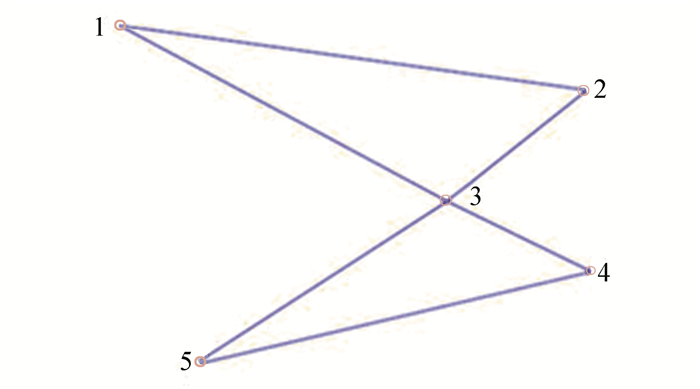
The multi-agent network formed by 5 agents is shown in Fig. 1. The agent aims to optimize velocities while minimizing the function
|
Fig.1 Communication network |
| $ \mathit{\boldsymbol{A}} = \left( {\begin{array}{*{20}{l}} 0&1&1&0&0\\ 1&0&1&0&0\\ 1&1&0&1&1\\ 0&0&1&0&1\\ 0&0&1&1&0 \end{array}} \right) $ |
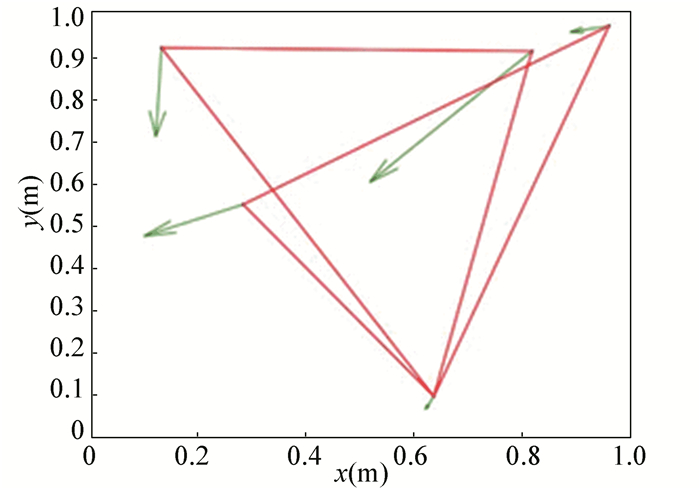
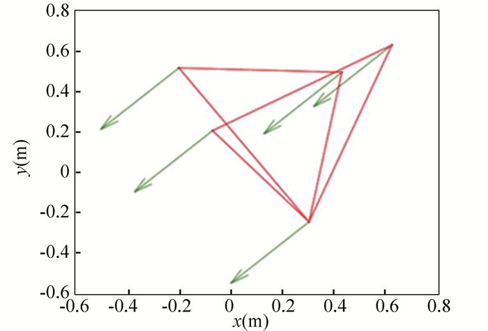
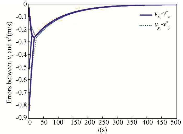
For the system (2)-(3), the nonlinear function is designed by f(vi) =ωvisinvi. This study randomly chose the initial velocity of each agent and marked it with dots. The initial status of the agent is presented in Fig. 2, where the full line between the two dots represents the path of the adjacent agent, while the arrow represents the motion direction of the agent. The final stable state of the agents is shown in Fig. 3. The error between the different velocity components and the optimal velocity is illustrated by Fig. 4, and the error curves of different velocity components are represented by different lines. The graph shows that the velocities reached the optimal velocity.
|
Fig.2 Initial configuration of agents |
|
Fig.3 Final configuration of agents |
|
Fig.4 Errors between agents and the optimal velocity |
The multi-agent network was formed by 10 agents. The adjacency matrix of the considered network graph is distributed by
| $ \mathit{\boldsymbol{A}} = \left( {\begin{array}{*{20}{l}} 0&1&1&0&0&1&1&0&1&1\\ 1&0&1&0&0&1&0&1&1&0\\ 1&1&0&1&1&0&1&1&0&1\\ 0&0&1&0&1&1&0&0&1&0\\ 0&0&1&1&0&1&0&1&0&1\\ 1&1&0&1&1&0&1&0&0&1\\ 1&0&1&0&0&1&0&1&1&0\\ 0&1&1&0&1&0&1&0&0&1\\ 1&1&0&1&0&0&1&0&0&1\\ 1&0&1&0&1&1&0&1&1&0 \end{array}} \right) $ |
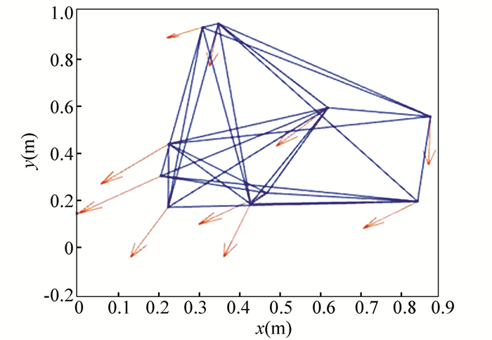
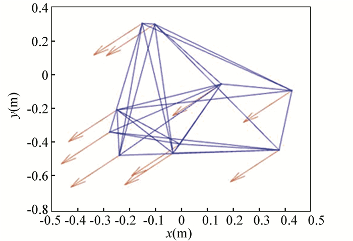
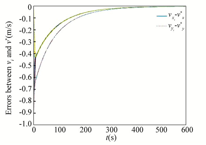
In this part, we select 10 agents which shows that the system can still achieve a stable state and velocities of the agents can reach the optimal velocity. The initial status of the agent is presented in Fig. 5, where the full line between the two dots represents the path of the adjacent agent, while the arrow represents the motion direction of the agent. The final stable state of the agents is shown in Fig. 6. The error between the different velocity components and the optimal velocity is illustrated by Fig. 7, and the error curves of different velocity components are represented by different lines.
|
Fig.5 Initial configuration of agents |
|
Fig.6 Final configuration of agents |
|
Fig.7 Errors between agents and the optimal velocity |
5 Conclusions
This study presented a distributed rule for heterogeneous systems. The optimization rule solved both consensus and optimization. First, the consensus issue was achieved for the second-order heterogeneous system, which is a more general and realistic system in accordance with Lyapunov stability theory and non-smooth analysis. Subsequently, it was shown that velocities of all agents were asymptotically optimal while minimizing the total cost function. Finally, to be recognized for the theoretical results, a simulation case was introduced. It is noteworthy that undirected topology plays an essential role.
| [1] |
Gao L X, Zhang J J, Chen W H. Second-order consensus for multiagent systems under directed and switching topologies. Mathematical Problems in Engineering, 2012(1): 58-80. DOI:10.1155/2012/273140 (  0) 0) |
| [2] |
Li X, Wu H, Yang Y. Consensus of heterogeneous multiagent systems with arbitrarily bounded communication delay. Mathematical Problems in Engineering, 2017, 1-6. DOI:10.1155/2017/5679073 (  0) 0) |
| [3] |
San B B, Sun X Y, Wu Y. Multi-objective optimization of membrane structures based on Pareto Genetic Algorithm. Journal of Harbin Institute of Technology (New Series), 2010, 17(5): 622-630. DOI:10.11916/j.issn.1005-9113.2010.05.005 (  0) 0) |
| [4] |
Bi X J, Zhang L, Cang Y. Constrained optimization algorithm based on double populations. Journal of Harbin Institute of Technology (New Series), 2016, 23(2): 66-71. DOI:10.11916/j.issn.1005-9113.2016.02.010 (  0) 0) |
| [5] |
Yuan D, Xu S, Zhao H. Distributed primal-dual subgradient method for multiagent optimization via consensus algorithms. IEEE Transactions on Systems, Man, and Cybernetics, Part B (Cybernetics), 2011, 41(6): 1715-1724. DOI:10.1109/TSMCB.2011.2160394 (  0) 0) |
| [6] |
Yi P, Hong Y. Quantized subgradient algorithm and data-rate analysis for distributed optimization. IEEE Transactions on Control of Network Systems, 2014, 1(4): 380-392. DOI:10.1109/tcns.2014.2357513 (  0) 0) |
| [7] |
Tsitsiklis J, Bertsekas D, Athans M. Distributed asynchronous deterministic and stochastic gradient optimization algorithms. IEEE Transactions on Automatic Control, 1986, 31(9): 803-812. DOI:10.1109/TAC.1986.1104412 (  0) 0) |
| [8] |
Li H, Huang C, Chen G, et al. Distributed consensus optimization in multiagent networks with time-varying directed topologies and quantized communication. IEEE Transactions Cybernetics, 2017, 47(8): 2044-2057. DOI:10.1109/TCYB.2017.2681119 (  0) 0) |
| [9] |
Nedic A, Ozdaglar A, Parrilo P A. Constrained consensus and optimization in multi-agent networks. IEEE Transactions on Automatic Control, 2010, 55(4): 922-938. DOI:10.1109/tac.2010.2041686 (  0) 0) |
| [10] |
Wang J, Elia N. A control perspective for centralized and distributed convex optimization. Proceedings of 2011 50th IEEE Conference on Decision and Control and European Control Conference. Piscataway: IEEE, 2011, 3800-3805. DOI:10.1109/CDC.2011.6161503 (  0) 0) |
| [11] |
Gharesifard B, Cortés J. Distributed continuous-time convex optimization on weight-balanced digraphs. IEEE Transactions on Automatic Control, 2014, 59(3): 781-786. DOI:10.1109/TAC.2013.2278132 (  0) 0) |
| [12] |
Kia S S, Cortés J, Martínez S. Distributed convex optimization via continuous-time coordination algorithms with discrete-time communication. Automatica, 2015, 55: 254-264. DOI:10.1016/j.automatica.2015.03.001 (  0) 0) |
| [13] |
Zhao Y, Liu Y F, Wen G H, et al. Distributed optimization for linear multiagent systems: Edge-and node-based adaptive designs. IEEE Transactions on Automatic Control, 2017, 62(7): 3602-3609. DOI:10.1109/TAC.2017.2669321 (  0) 0) |
| [14] |
Wang X, Hong Y. Finite-time consensus for multi-agent networks with second-order agent dynamics. IFAC Proceedings Volumes, 2008, 41(2): 15185-15190. DOI:10.3182/20080706-5-kr-1001.02568 (  0) 0) |
| [15] |
Wang L, Sun S, Xia C. Finite-time stability of multi-agent system in distributed environment. Nonlinear Dynamics, 2012, 67(3): 2009-2016. DOI:10.1007/s11071-011-0125-0 (  0) 0) |
| [16] |
George K, Subramanian K. Adaptive control of a class of nonlinear time-varying systems with multiple models. Control Theory and Technology, 2016, 14(4): 323-334. DOI:10.1007/s11768-017-6095-0 (  0) 0) |
| [17] |
Zheng Y, Wang L. Consensus of heterogeneous multi-agent systems without velocity measurements. International Journal of Control, 2012, 85(7): 906-914. DOI:10.1080/00207179.2012.669048 (  0) 0) |
| [18] |
Chung F R K. Spectral Graph Theory. California, USA: American Mathematical Society, 1997.
(  0) 0) |
| [19] |
Filippov A F. Differential Equations with Discontinuous Righthand Side. Dordrecht: Springer, 1988.
(  0) 0) |
| [20] |
Paden B, Sastry S. A calculus for computing Filippov's differential inclusion with application to the variable structure control of robot manipulators. IEEE Transactions on Circuits and Systems, 1987, 34(1): 73-82. DOI:10.1109/TCS.1987.1086038 (  0) 0) |
| [21] |
Shevitz D, Paden B. Lyapunov stability theory of nonsmooth systems. Proceedings of the 32nd IEEE Conference on Decision and Control, 1993, 1: 416-421. DOI:10.1109/CDC.1993.325114 (  0) 0) |
| [22] |
Boyd S, Vandenberghe L, Faybusovich L. Convex optimization. IEEE Transactions on Automatic Control, 2006, 51(11): 1859-1865. DOI:10.1109/TAC.2006.884922 (  0) 0) |
 2020, Vol. 27


