2. KEJIE Machinery Automation Co., Ltd., Jiangmen 529030, Guangdong, China
The development of manufacturing industry has increased the requirements for NC machining, which plays a vital role in manufacturing. The accuracy of product is an important indicator of NC machining. However, there are still some problems in the traditional NC machining in large batch processing of a single workpiece represented by 3C products such that it is only repetitive control and every processing is entirely new. When accuracy is not increased, the error of each batch remains the same, and the error data in production are not effectively utilized to improve the accuracy of subsequent production.
Iterative learning control[1] is a "human learning" approach that adopts the strategy of "learning in repetitive operation", which can gradually adjust the control input, add appropriate compensation amount to controller at the appropriate time, and improve the accuracy of the system. In 1984, Arimoto et al.[2] first proposed the theory of iterative learning control and demonstrated the method, which created a new research direction of control method. Iterative learning consists of open-loop structure, closed-loop structure, and open-closed-loop structure, among which the division of open-closed-loop structure is based on the use of the learning error during current or previous cycle. Since iterative learning is for multiple operations of the same trajectory, it is also extended to the higher-order iterative[3], i.e., iterative learning that uses multiple running errors, such as K times, K-1 times, and K-2 times. Chen et al.[4] verified that the higher-order algorithm is superior to the first-order iterative learning algorithm and the delay of the system does not affect the stability of the iterative learning algorithm. Open-loop iteration is similar to "feedforward" control, which does not affect the stability of the system. However, the open-loop iterative structure is more suitable for solving the problem because of its poor transience inherent in the iterative process. Li[5] considered that high-order iterative learning control uses more historical tracking error information, which proves that the PD high-order iterative learning control algorithm adopted in the nonlinear and time-varying system converges fast. Learning law is an algorithm that uses errors in the process of learning, which is the core of the study of iterative learning. In addition to the D type learning law, Arimoto[2] proposed other PID type iterative learning laws, which are effective and widely used.
On the basis of filter, Bien and Xu[6] introduced iterative learning control method. Feedback signal was first filtered and applied to learning law to avoid the effect of noise on the iterative convergence process. Since the acquisition of feedback signal may be influenced by noise as mentioned in Refs. [7-10], in which filter was introduced to suppress the bad transient phenomenon, the causes of this phenomenon were analyzed in time domain and frequency domain. It is the accumulation of high-frequency noise that causes the system divergence in the process of iterations. To solve this problem, some researchers proposed to filter the collected signal to eliminate the influence of noise. Li et al.[11] designed an iterative learning method based on zero-phase filter for the injection speed control of injection molding machine, so the learning control algorithm is monotone convergent. Tsai et al.[12] put forward the EMD[13] decomposition error signal, which eliminates the divergence caused by the system, avoids the local divergence of the system, and improves the tracking accuracy of the system.
Elci et al.[14] put forward a method according to experience and gradually adjusted the filter frequency to determine the cutoff-frequency of the filter cutoff, in which high-frequency noise low-pass filter design is reasonable. Zhang et al.[15] proposed a new method for Wigner of error signal time-frequency analysis to identify the current dominant frequency components of error, and the filter design is reasonable. To improve the performance of the system, Rotariu et al.[16] added a time-varying robust filter into deterministic disturbance, in which the avoided noise was amplified. Huang and Chen[17] proposed a wavelet transform based filter to add to the feedforward part to reduce the adverse effects of unlearning dynamics and enhance the robustness of the system.
The use of low-pass filter may lose the learning of some high-frequency effective information. As this research is slightly inadequate, especially in combination with the input of velocity planning in motion control, reasonable filter was designed to make the research more practical. Therefore, a switchable filter was used, and cutoff-frequency was ensured through the frequency analysis of input signal path. Multiple low-pass filter in different stages of the operation cycle was utilized with different cutoff-frequencies in different time to suppress the high frequency noise and select the high frequency signal which are useful in the learning, which can realize the monotone convergence performance and system robustness.
To sum up, in this paper, an iterative learning controller is designed based on the actual needs of motion control field, which can improve the accuracy of machining in single workpiece processing. When applying the iterative algorithm to actual numerical control system, the best results can be obtained by considering the characteristics of the controlled object and the actual input. The rest of this paper is organized as follows. Section 2 and Section 3 introduce the principle of iterative learning and the design of open-loop iterative learning controller, respectively. In Section 4, based on iterative learning controller and switch type iterative learning mechanism, the divergence problem of local error is solved through the filter design. In Section 5, the design of the switchable filter is proposed to further improve the system performance, and experiments are presented in Section 6.
2 Iterative Learning Control AlgorithmDifferent from traditional feedback control, the current control point of interpolation point is determined by the error of the last time. The control point of the current interpolation point in iterative learning is composed of the current time controlled quantity at the last time and the current time error in the last iteration.
Control structures are divergent through the different uses of controlled quantity and error. There are two main types of iterative learning control structure, the series structure and the parallel structure[18]. The series structure changes the reference input signal to optimize the input trajectory reasonably(Fig. 1), which is applicable to the case when commercial controller does not have direct access to modify the control signal. However, this method is modified outside the three loop control and the speed is slow. Because of the modification of input, the speed of the planning input will be greatly changed. Only when the compensation is reasonable can better control result be achieved.

|
Fig.1 Series structure (modified reference input)[18] |
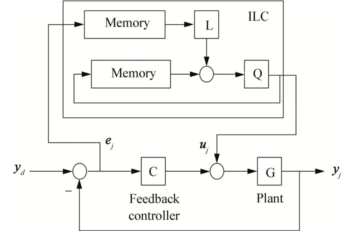
The use of parallel structure error is shown in Fig. 2. With the superposition of similar feedforward control output and feedback controller, the overall control amount of the controller to regulate the amount of feedback and feedforward control is composed of force control, which modifies the control input way more quickly, and can timely and effectively update the control input, and whose control effect is more significant.
|
Fig.2 Parallel structure (modification control)[18] |
The addition of the feedforward part of control input can improve the fast response of the system. After dynamically adjusting the overall control input, the system error can be quickly and monotonously converged to the ideal range.
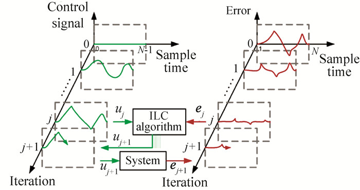
As shown in Fig. 3, each signal can be divided into a time axis and an iterative axis. At the initial iteration, the iterative part of the control amount is 0, and the iteration starts to play an important role at the second iteration.
| $ \mathit{\boldsymbol{u}}{\mathit{\boldsymbol{}}_{j + 1}}\left( t \right){\rm{ }} = \mathit{\boldsymbol{ u}}{_j}\left( t \right){\rm{ }} + \mathit{\boldsymbol{ Le}}{_j}\left( t \right) $ | (1) |
|
Fig.3 Control input and error diagram of iterative learning control[18] |
where
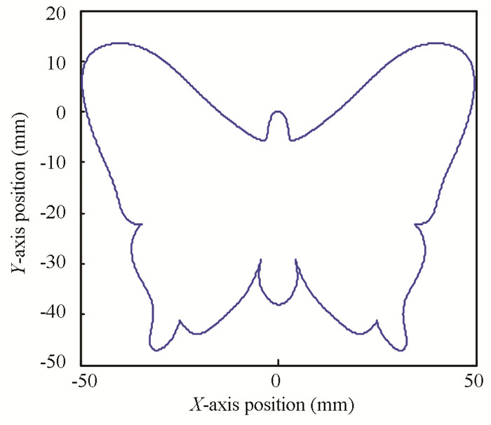
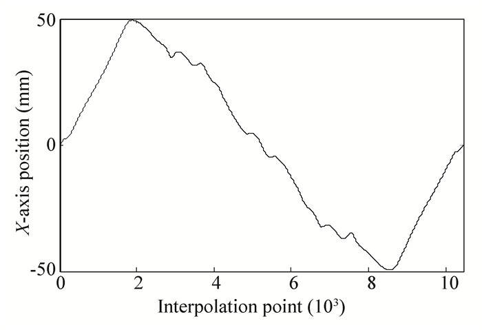
In this study, the control goal is to make the system follow the given input signal which is the actual trajectory in the motion control. Therefore, the butterfly trajectory was taken as an example to experiment with the single axis signal of the butterfly trajectory, and the trajectory and the X-axis signal are demonstrated in Figs. 4-5, and the relationship of X-axis between position and velocity is as shown in Fig. 6.
|
Fig.4 Butterfly input signal |
|
Fig.5 X-axis of the butterfly |
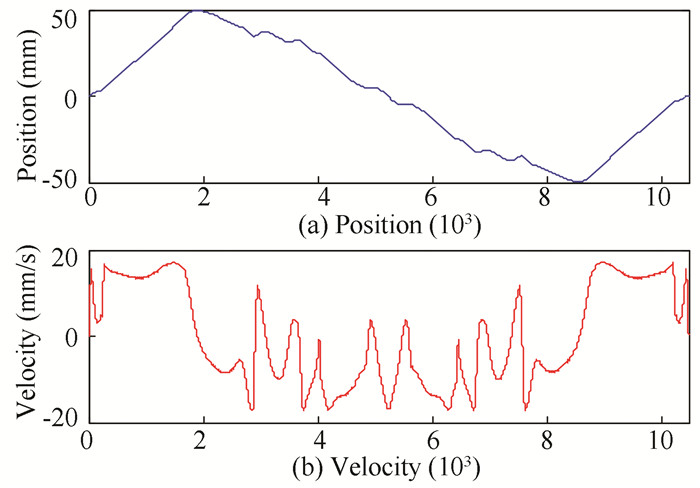
|
Fig.6 Position and speed information of input signal |
In actual processing, PID control with superposition speed feedforward can achieve good control effect, but desired result is not achievable when faced with complex trajectory signals.
It can be seen from Figs. 7-8 that the tracking error of the butterfly trajectory was reduced after the introduction of speed feedforward, and the maximum tracking error reduced from ± 0.060 mm to ± 0.018 mm. However, the accuracy could not be further improved because precision was limited in experimental conditions. In the case of complex trajectory in motion control, the feedback control effect of superposition speed feedforward had its limitations, which was solved by introducing an iterative learning mechanism in this study.
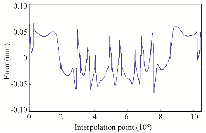
|
Fig.7 Feedback control error curve |
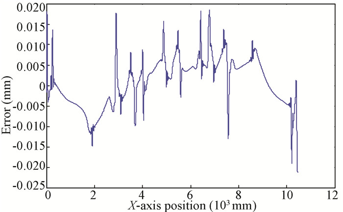
|
Fig.8 Tracking error with speed feedforward |
3.1 Selection of Iterative Learning Structure
In this paper, starting with the control layer, the control input was modified, so the iterative learning structure of the modified control type was selected. According to the error in control volume, it can be divided into open-loop iteration and closed-loop iteration. The open-loop iteration uses the error of the last time in the current operation, and the closed-loop iteration uses the error of the current time in the current operation. To ensure the appropriate amount of control is at the appropriate time, the open-loop iterative learning method was adopted in this paper.
Fig. 9 is an iterative learning block diagram for the practical application of servo system, in which the control amount is composed of two parts including feedback control and iterative learning control.
| $ \left\{ \begin{array}{l} \mathit{\boldsymbol{u}}{_j}\left( k \right){\rm{ }} = \mathit{\boldsymbol{ w}}{\mathit{\boldsymbol{}}_j}\left( k \right){\rm{ }} + \mathit{\boldsymbol{ C}}{\rm{ }}\left( z \right){\rm{ }}\mathit{\boldsymbol{e}}{\mathit{\boldsymbol{}}_j}\left( k \right)\\ \mathit{\boldsymbol{w}}{_j}\left( k \right){\rm{ }} = \mathit{\boldsymbol{ w}}{_{j - 1}}\left( k \right) + \phi \mathit{\boldsymbol{e}}{_{j - 1}}\left( k \right) \end{array} \right. $ | (2) |

|
Fig.9 Iterative learning structure diagram of servo system |
where
Iterative learning control can deal with repetitive interference well, and the role of nonlinear links is considered to be repetitive interference. Fig. 10 demonstrates that the iterative learning control had a good control effect on the servo system with repetitive interference.
|
Fig.10 Verification of the effect of iterative learning on repetitive interference suppression |
The elliptic curve in Fig. 10 represents disturbance, and the iterative learning control input was the same with the disturbance, both of which were added in the output of position loop controller. The feedback controller is mainly responsible for maintaining the stability of the inner part, and the iteration can gradually inhibit the repetitive disturbance. For the interference of repetitive control, when it suddenly increased, the iterative operation gradually converged to a relatively stable state, which was also accompanied by introducing errors in the interference, and then it gradually decreased with no further impacts on the system.
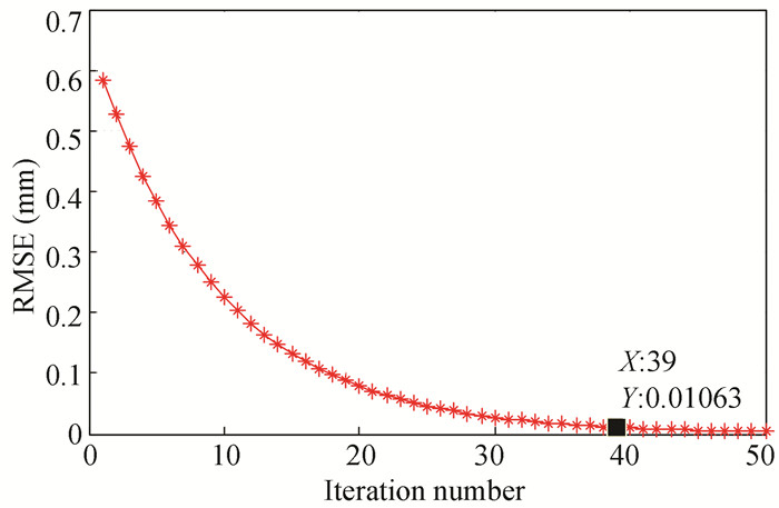
Repetitive disturbances were introduced at 1.25 s (the 625th interpolation point), when the error changed greatly. As shown in Fig. 11, such adverse change could not be dealt with in time by simple feedback control. The variation trend of the error signal is illustrated in Fig. 12, in which the error increased sharply to a larger value, leading to the increase of the overall error amplitude. After the iterative learning was introduced, although the errors in the first few changes were more violent, the control volume was gradually optimized with the iteration. After 39 iterations, the root-mean-square error(RMSE) could converge to 0.01 mm.

|
Fig.11 Repetitive disturbance error curve |
|
Fig.12 RMSE curve with iterations |
In response to this situation, open-loop iterative learning was used to verify the effectiveness.
It can be seen from Fig. 13 that iterative learning control could gradually reduce the variation of control variables introduced by disturbance through adjusting the control input, and the error gradually converged to less than 5 μm with iteration. The control input of the iterations increase with the increase of the iteration numbers (Fig. 13).

|
Fig.13 Iteration part of the control volume curve |
The iterative learning control gradually adjusted the control amount of iteration to increase it to the desired control range, and then it gradually suppressed the error caused by the disturbance. The more the iterations are, the smaller the impact of disturbance is, and the smaller the system tracking error is.
4 Filter-Based Iterative Learning Controller DesignIn simulation and experiment, there is a phenomenon that in the position control, the tracking error is always monotonically convergent, although it will eventually converge to a reasonable extent. Though such instability phenomenon occurs during the iterative operation, rather than at the start of the iteration, the error in this process is still unacceptable. In experiment, the sharp increase of the control amount will exceed the limit of the saturation of the driver, causing the driver to alarm and the motor to rotate at a high speed, thus posing a potential safety hazard.
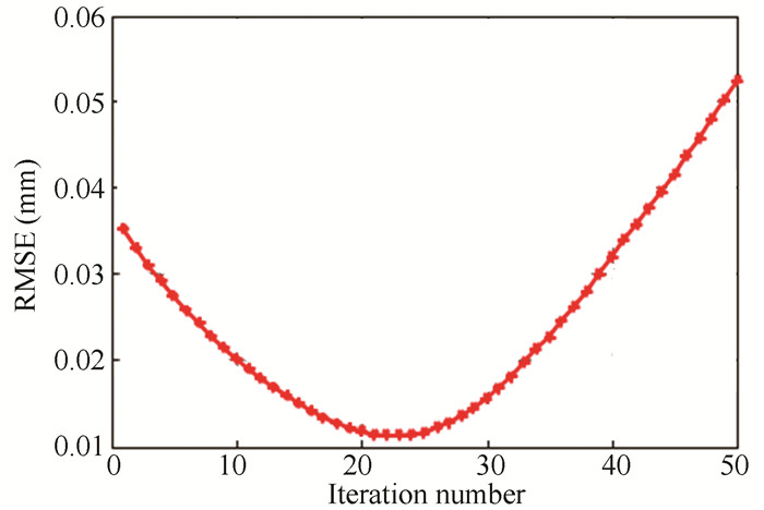
Ideally, the RMSE and the overall error should be reduced as the number of iterations increases. Because of the iterative learning structure which was utilized to modify and control the quantum iteration, the iterative partial control input became gradually dominated (close to the desired control), and the iterative mechanism amplified the influence of high-frequency noise. With the increase of iterative operation, the accumulation of high-frequency noise gradually had a negative impact, which led us to think about how to achieve monotonous and rapid convergence.
As shown in Fig. 14, in the simulation, the RMSE gradually decreased with the iteration in the initial stage, while from the 22nd iteration, the error gradually increased.
|
Fig.14 Simulation of RMSE with iteration |
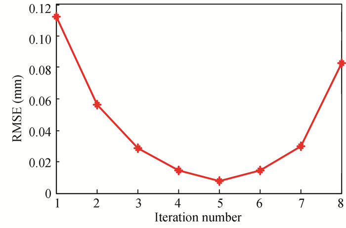
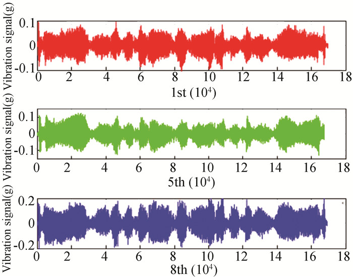
According to Fig. 15, the same situation occurred during the experiment. At the sixth iteration, the RMSE of the system increased, indicating that the systematic error is no longer monotonically convergent, which should be analyzed. A similar situation can be observed from the vibration signal (Fig. 16).
|
Fig.15 Variation of RMSE in the experiment with iteration |
|
Fig.16 Vibration signal with iterative curve |
It can be seen from Fig. 16 that the overall trend of the system vibration signal did not change as the amplitude gradually increased, indicating that the system was at a poor transient state. In addition, in the experiment, the larger the parameters of the position loop controller were, the more divergent the error would be, so the vibration phenomenon would make the experiment difficult to continue.
With identification, the state space expression of the system can be expressed as follows:
| $ \left\{ \begin{array}{l} \begin{array}{*{20}{c}} \begin{array}{l} \mathit{\boldsymbol{x}}(k + 1) = \left[ {\begin{array}{*{20}{c}} {2.8500}&{ - 1.3500}&{0.8502}\\ 2&0&0\\ 0&{0.5}&0 \end{array}} \right]\mathit{\boldsymbol{x}}(k) + \\ \;\;\;\;\;\;\;\;\;\;\;\;\;\;\;\;\;\left[ {\begin{array}{*{20}{c}} {0.25}\\ 0\\ 0 \end{array}} \right]\mathit{\boldsymbol{u}}(k) + \mathit{\boldsymbol{\omega }}(k)\;\;\;\;\;\;\;\;\;\;\;\;\; \end{array}\\ \end{array}\\ \mathit{\boldsymbol{y}}(k) = \left[ {\begin{array}{*{20}{c}} {0.19000}&0&{ - 0.01899} \end{array}} \right]\mathit{\boldsymbol{x}}(k) \end{array} \right. $ | (3) |
where A is the system matrix, x is state vector, u is control input, y is system output, and w is disturbance. Iteration learning law is described as
| $ \mathit{\boldsymbol{u}}{\mathit{\boldsymbol{}}_{j + 1}}\left( t \right){\rm{ }} = \mathit{\boldsymbol{ u}}{_j}\left( t \right){\rm{ }} + {\rm{ }}\mathit{\boldsymbol{Le}}{_j}\left( t \right) $ | (4) |
where j is iteration number, and L is learning gain matrix. When choosing a fixed learning gain, its characteristic value is a fixed-value
| $ \mathit{\boldsymbol{e}}{\mathit{\boldsymbol{}}_j} = \left( {\mathit{\boldsymbol{I }} - {\rm{ }}\mathit{\boldsymbol{PL}}} \right)\mathit{\boldsymbol{e}}{_{j - 1}} $ | (5) |
The P matrix composed of Markov parameters is described in Eq.(6) as
| $ \boldsymbol{P}=\left[\begin{array}{ccccc} \boldsymbol{C B} & 0 & 0 & \cdots & 0 \\ \boldsymbol{C A B} & \boldsymbol{C B} & 0 & \cdots & 0 \\ \boldsymbol{C A}^{2} \boldsymbol{B} & \boldsymbol{C A B} & \boldsymbol{C B} & \cdots & 0 \\ \vdots & \vdots & \vdots & \vdots & \vdots \\ \boldsymbol{C A}^{p-1} \boldsymbol{B} & \boldsymbol{C A}^{p-2} \boldsymbol{B} & \boldsymbol{C A}^{p-3} \boldsymbol{B} & \cdots & \boldsymbol{C B} \end{array}\right] $ | (6) |
where
In the time domain, only sufficient convergence condition can be provided, which cannot explain the phenomenon of partial divergence of error well enough, making it necessary to analyze from Z domain.
Therefore, the system was transformed into Z domain as
| $ \mathit{\boldsymbol{Y}}{_j}\left( z \right){\rm{ }} = {\rm{ }}\mathit{\boldsymbol{G}}{\rm{ }}\left( z \right){\rm{ }}\mathit{\boldsymbol{U}}{_j}\left( z \right){\rm{ }} + {\rm{ }}\mathit{\boldsymbol{C}}{\rm{ }}{\left( {z{\rm{ }}\mathit{\boldsymbol{I}} - \mathit{\boldsymbol{A}}{\rm{ }}} \right)^{ - 1}}\mathit{\boldsymbol{W}}{\rm{ }}\left( z \right) $ | (7) |
where
| $ \mathit{\boldsymbol{E}}{_j}\left( z \right){\rm{ }} = \frac{{{\rm{ }}1 - \phi z{\rm{ }}\mathit{\boldsymbol{G}}{\rm{ }}\left( z \right){\rm{ }} + {\rm{ }}\mathit{\boldsymbol{C}}{\rm{ }}\left( z \right){\rm{ }}\mathit{\boldsymbol{G}}{\rm{ }}\left( z \right)}}{{1 + {\rm{ }}\mathit{\boldsymbol{C}}{\rm{ }}\left( z \right){\rm{ }}\mathit{\boldsymbol{G}}{\rm{ }}\left( z \right)}}\mathit{\boldsymbol{ E}}{_{j - 1}}\left( z \right) $ | (8) |
System monotonous convergence condition is
| $ \left| {1 - \frac{{{\rm{ }}\phi z{\rm{ }}\mathit{\boldsymbol{G}}{\rm{ }}\left( z \right){\rm{ }}}}{{1 + {\rm{ }}\mathit{\boldsymbol{C}}{\rm{ }}\left( z \right){\rm{ }}\mathit{\boldsymbol{G}}{\rm{ }}\left( z \right)}}} \right| < 1 $ | (9) |
At each iteration, if the system satisfies the monotone convergence condition (9), the system will be monotonically convergent, thus strict demands should be placed on the frequency of the signal. The high-frequency component of the signal that exceeds the critical frequency led to the error to increase inversely with iteration.
The learning law
Iterative learning control can effectively restrain the repetitive interference, while it cannot effectively suppress this part of signal because it has little inhibitory effect on high-frequency noise accumulation. Therefore, without filter learning system, the system would accumulate non-repetitive high-frequency random interference signals along the iteration axis, thus the local tracking error in the iterative process would first decrease and then increase.
Here are the steps for a digital filter design:
1) Determine the type of the filter (such as low-pass filter) on the basis of needs;
2) According to the requirements, decide the pass frequency and cutoff-frequency, as well as the passband ripple coefficient and stopband ripple coefficient;
3) Filter Infinite Impulse Response (IIR) butterworth type of filter according to the parameters of the first design of the analog filter;
4) Apply the "impulse response invariant method" analog filter to a digital filter.
Commonly used low-pass filter mathematical expressions are described by the transfer function denominator and molecular vector A, B, the input vector X filter, and the filter output vector Y. The low-pass filter is described as
| $ \begin{array}{l} \mathit{\boldsymbol{y }}\left( n \right){\rm{ }} = {\rm{ }}\mathit{\boldsymbol{b}}{\rm{ }}\left( 1 \right) \cdot \mathit{\boldsymbol{x}}{\rm{ }}\left( n \right) + \ldots + {\rm{ }}\mathit{\boldsymbol{b}}{\rm{ }}\left( {{N_b} + 1} \right){\rm{ }}\cdot{\rm{ }}\mathit{\boldsymbol{x }}\left( {n - {N_b}} \right){\rm{ }} - \\ \;\;\;\;\;\;\;\mathit{\boldsymbol{a }}\left( 2 \right) \cdot \mathit{\boldsymbol{y}}{\rm{ }}\left( {n - 1} \right) - \ldots - {\rm{ }}\mathit{\boldsymbol{a }}\left( {{N_a} + 1} \right){\rm{ }}\cdot{\rm{ }}\mathit{\boldsymbol{y}}{\rm{ }}(n - {N_a}) \end{array} $ | (10) |
This paper uses a fourth-order filter to process data, and the parameters are
| $ \begin{array}{*{20}{l}} {\mathit{\boldsymbol{a }} = {\rm{ }}[1, {\rm{ }} - 2.8531, {\rm{ }}2.7167, {\rm{ }} - 0.8633]}\\ {\;\;\;\;\mathit{\boldsymbol{b }} = {\rm{ }}[0, {\rm{ }}0.00018896, {\rm{ }}0.00017992]} \end{array} $ |
with the cutoff-frequency of 10 Hz.
In control system, the overshoot of the system might become larger because of a cumulative change in phase, thus the dynamic response capability of the system was reduced. Therefore, zero-phase-filter was applied and processed twice to filter the signal. Make the signal pass forward to obtain the output signal, and then pass back through filtering. The phase lag caused by the forward filter was offset by the reverse pass filter, and the process can be described by Eq.(11), where x (n) is the input signal, y (n) is the output signal, y4(n) is the final output signal, h (n) is the filter, and N represents the total data points.
| $ \left\{ \begin{array}{l} \mathit{\boldsymbol{y}}{_1}\left( n \right){\rm{ }} = \mathit{\boldsymbol{ x}}{\rm{ }}\left( n \right){\rm{ }}\mathit{\boldsymbol{h}}{\rm{ }}\left( n \right)\\ \mathit{\boldsymbol{y}}{_2}\left( n \right){\rm{ }} = {\rm{ }}\mathit{\boldsymbol{y}}{_1}\left( {N - 1 - n} \right)\\ \mathit{\boldsymbol{y}}{\mathit{\boldsymbol{}}_3}\left( n \right){\rm{ }} = \mathit{\boldsymbol{ y}}{_2}\left( n \right){\rm{ }}\mathit{\boldsymbol{h}}{\rm{ }}\left( n \right)\\ \mathit{\boldsymbol{y}}{_4}\left( n \right){\rm{ }} = {\rm{ }}\mathit{\boldsymbol{y}}{_3}\left( {N - 1 - n} \right) \end{array} \right. $ | (11) |
Fig. 17 shows the structure of the simulation and experiment. First, determine the cutoff-frequency of the system, and then follow the steps to design the corresponding low-pass filter. Off-line mode was applied when each operation is over, the system goes back to zero gap, and the error is filtered. When the next iteration starts to run, the filtered error signal is added.

|
Fig.17 Filter-based iterative learning structure |
Fig. 18 demonstrates the monotonous convergence of the RMSE value with iteration, and no error divergence occurred again, which proved that the filter-based iterative learning structure could solve the problem of error divergence. In engineering practices, since the PID controller adjusts the parameter to be few and the regulating performance is good, PID controller is often utilized. However, experience is necessary for the adjustment of the controller parameters, which can make it adjust to more superior performance fast and accurately. The position loop feedback PID parameters were first roughly adjusted, and then the iterative control amount was superposed to achieve superior control performance. When the tracking accuracy reaches a reasonable threshold range, iteration stops, and the current amount as the ideal control is thus controlled. The flow chart of the process is shown in Fig. 19.

|
Fig.18 Simulation of RMSE with the iterative curve (filtered) |

|
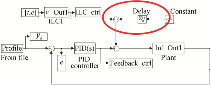
Fig.19 Switching mechanism of iterative learning |
Iteration requires a certain amount of calculation, so it should not be indefinitely carried out, which is not in line with the actual processing needs. Through this switch mechanism, better control accuracy can be achieved in a quick and easy way, and the control intelligent is increased.
The method was also used as a solution to avoid the divergence of iterative learning errors. The system can observe the changes of error in real-time during the system running. In simulation and experiment, as the figure describes, when the error fell within the allowable range, the iteration switched with constant feedforward control amount as a compensation. With the stop of the iteration, the adverse effects of high-frequency noise would not be amplified. However, this is a simple solution that even if the error is not within the allowable range, the iteration mechanism can be empirically closed before the divergence of the error. Although the error is no longer divergent, the processing is not ideal. To fundamentally solve the problem of running away from the error in the process of divergence, it is necessary to address the causes behind. To avoid the influence of poor transience, reasonable design of the low-pass filter can eliminate the high-frequency noise that causes the divergence of the system. However, this brings the problem that when the complex input high-frequency signal is valid in some segments, the low-pass filter to get rid of this part of high-frequency effective information is not successfully added to the learning, so it is difficult to further improve the convergence accuracy. Although the introduction of off-line low-pass filter is not the best solution of this issue, it is valid in this problem. For the input signal and error information, the time-frequency analysis was carried out to find the effective high-frequency signal of the time section, where the cutoff-frequency can be changed. The design of the entire operation of the switchable low-pass was filtered, which further improved the convergence performance.
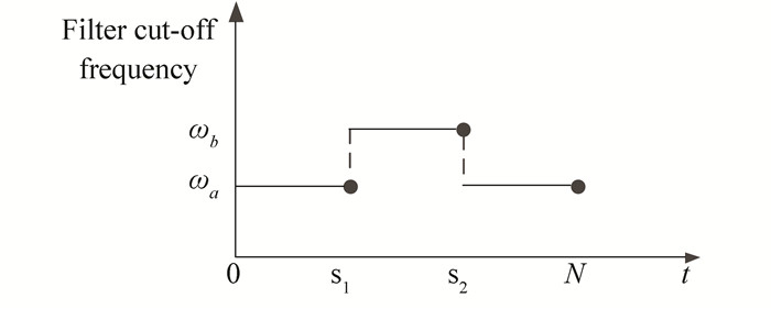
5 Switchable Filter DesignThe expected trajectory often contains more frequency information. The low-pass filter designed in Section 3 can filter out some of the high-frequency effective information, while it makes the convergence accuracy hard to be further improved in the high-frequency distributed time segment. Through modifying the controlled quantity of the iterative learning control by introducing a low-pass filter, the last tracking error was filtered off-line, which can solve the problem of the divergence of the tracking error during operation. Based on the above filter, combined with the analysis of the input trajectory and the error signal, higher cutoff-frequency was selected in some sections(Fig. 20).
|
Fig.20 Schematic of switched filter |
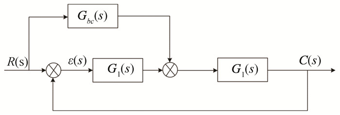
The system uses different cutoff-frequencies wa and wb in different time segments, and selects a low-pass filter with cutoff-frequency wa in the time segment [0, S1], cutoff-frequency wb in the time segment [S1, S2], and cutoff-frequency wa of the low-pass filter, which can be expressed by Eq.(12). Furthermore, the switchable filter was compensated by adding feedforward channel from the structure diagram and transfer function of the system (Fig. 21). For Eqs.(13) and (14), by comparing the transfer function before and after the change, the pole of the system did not change and the system remained stable.
| $ \begin{array}{l} Q = \\ \left\{ {\begin{array}{*{20}{l}} {{b_1}(1) \cdot \mathit{\boldsymbol{x}}(n) + \cdots + {b_1}\left( {{N_b} + 1} \right) \cdot \mathit{\boldsymbol{x}}\left( {n - {N_b}} \right) - {a_1}(2) \cdot }\\ {\;\;\;\;\;\;\;\mathit{\boldsymbol{y}}(n - 1) - \cdots - {a_1}\left( {{N_a} + 1} \right) \cdot \mathit{\boldsymbol{y}}\left( {n - {N_a}} \right),t \in \left[ {0,{S_1}} \right)}\\ {{b_2}(1) \cdot \mathit{\boldsymbol{x}}(n) + \cdots + {b_2}\left( {{N_b} + 1} \right) \cdot \mathit{\boldsymbol{x}}\left( {n - {N_b}} \right) - {a_2}(2)}\\ {\;\;\;\;\;\;\;\mathit{\boldsymbol{y}}(n - 1) - \cdots - {a_2}\left( {{N_a} + 1} \right) \cdot \mathit{\boldsymbol{y}}\left( {n - {N_a}} \right),t \in \left[ {0,{S_1}} \right)}\\ {{b_3}(1) \cdot \mathit{\boldsymbol{x}}(n) + \cdots + {b_3}\left( {{N_b} + 1} \right) \cdot \mathit{\boldsymbol{x}}\left( {n - {N_b}} \right) - {a_3}(2)}\\ {\;\;\;\;\;\mathit{\boldsymbol{y}}(n - 1) - \cdots - {a_3}\left( {{N_a} + 1} \right) \cdot \mathit{\boldsymbol{y}}\left( {n - {N_a}} \right),t \in \left[ {0,{S_1}} \right)} \end{array}} \right. \end{array} $ | (12) |
|
Fig.21 Frame of the system |
where parameters b1 and a1, b2 and a2, and b3 and a3 represent the cutoff-frequency 10 Hz, 50 Hz, and 10 Hz, respectively.
| $ {\phi _1} = {\rm{ }}\frac{{\mathit{\boldsymbol{G}}{_1}\left( s \right){\rm{ }}\mathit{\boldsymbol{G}}{_2}\left( s \right){\rm{ }}}}{{1 + {\rm{ }}\mathit{\boldsymbol{G}}{_1}\left( s \right){\rm{ }}\mathit{\boldsymbol{G}}{_2}\left( s \right)}} $ | (13) |
| $ {\phi _2} = \frac{{{\rm{ }}\mathit{\boldsymbol{G}}{\mathit{\boldsymbol{}}_1}\left( s \right){\rm{ }}\mathit{\boldsymbol{G}}{_2}\left( s \right) + {\rm{ }}\mathit{\boldsymbol{G}}{_2}\left( s \right){\rm{ }}\mathit{\boldsymbol{G}}{_{bc}}\left( s \right)}}{{1 + {\rm{ }}\mathit{\boldsymbol{G}}{_1}\left( s \right){\rm{ }}\mathit{\boldsymbol{G}}{_2}\left( s \right)}}{\rm{ }} $ | (14) |
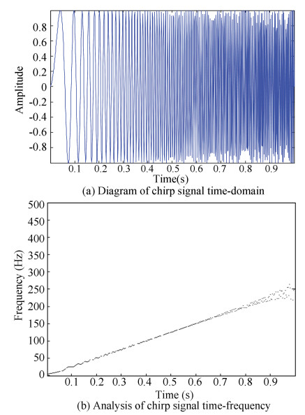
The filter in the same iteration process have different cutoff-frequencies in different time intervals, and it is suitable for such situations when the system is in different time intervals with useful high-frequency information because of the response characteristics or the specific system. The time-frequency analysis of the input trajectory signal was carried out to obtain its frequency information to facilitate the iterative learning critical divergence frequency and the effective frequency of information between the design of a reasonable switchable filter. Hilbert transform can be considered as a special fast Fourier transform. More prominent signal time-frequency changed in the specific circumstances can give us a new perspective to analyze signal changes. Based on the above analysis, the following examples verified the effectiveness of the time-frequency analysis. Chirp is a signal, whose signal frequency is strictly mathematically related to time and is well suited to represent the relationship between time and frequency.
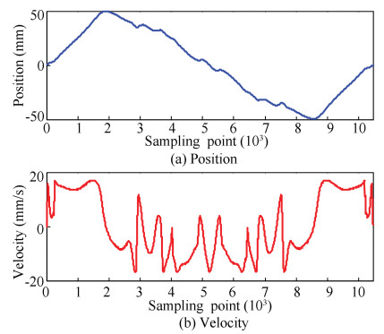
It can be found in Fig. 22 that the frequency distribution of the chirp signal provided a true description of the frequency of the dominant signal at each moment, showing that it is a reasonable method to analyze the input signal. The applied input track is still the X-axis information of the butterfly trajectory(Figs. 23-24), which present the position information of the track and the speed change.
|
Fig.22 Chirp signal time-frequency analysis |
|
Fig.23 Butterfly input signal corresponding to the X-axis position and speed |

|
Fig.24 Speed and error information (first cycle with no iteration) |
In simple feedback, the proportional control of the output voltage is analog, which is proportional to speed. Therefore, the trend of error is same to the trend of speed that large errors are in large places, and when the speed changes rapidly, the error changes in the same way, which is a common problem in the field of motion control. For complex trajectories, the effect of the commonly used PID control is not ideal, whereas iterative control can optimize the control effect. Therefore, the time-frequency analysis mentioned in the previous section was used to analyze the input signal and determine the cause of the error.
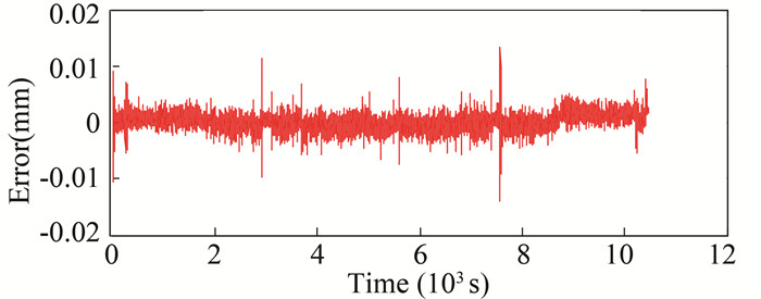
After 8 iterations, the overall error was greatly improved from 0.06 mm to 0.01 mm (Fig. 25), less than that without iterative feedback control.
|
Fig.25 Error information and speed information (iteration 8 times) |
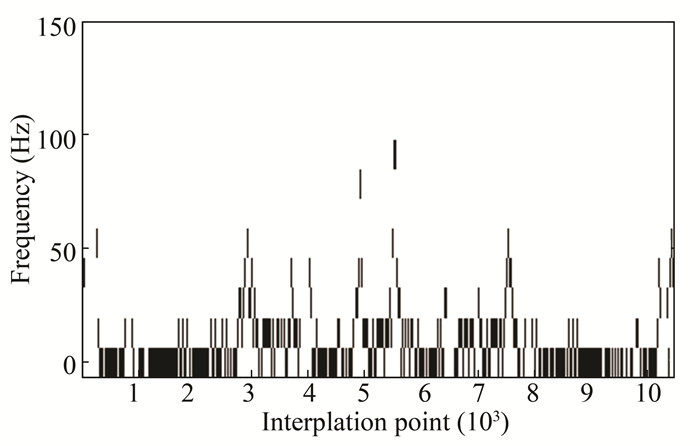
According to the time-frequency analysis of the input signal (Fig. 26), the instantaneous frequencies were higher near the interpolation points (2915, 5249, 6093, and 7576), so the error signal should be treated as special. The overall error converged to 0.01 mm, but the errors near the local points (corresponding to the 2915th and the 7576th interpolation points) would be significantly large.
|
Fig.26 Results of input signal time-frequency analysis |
Experiments show that even if the iteration continued, the error could not be improved and the learning performance was close to limit. By comparing error information and velocity time-frequency analysis, it can be found that the change of velocity was violent at the point of great error, where the input signal frequency was higher. To solve the bad transience, filter was utilized to remove this part of signal, resulting in a particular interval, and the accuracy could no longer be improved with iteration. Iterative learning control of switchable filters was proposed to further improve and optimize the accuracy of iterative learning control. First, input trajectory signal was analyzed to determine its frequency information. Then, the system was analyzed, and the corresponding cutoff-frequency was determined according to the system error divergence condition and the frequency information of trajectory with the reasonable cutoff-frequency of low-pass filter (Fig. 27). In this way, at each iteration interval, the designed switchable filter was used to filter the deviation signal between the planned position and the actual position, i.e., the error signal introduced into the iterative part was processed. This method not only avoids the divergence problem of error during the system iteration, but also improves the accuracy of the section when the error is large on the original basis. In the process of iteration to determine the changes of the overall error and the RMSE, when it is within a reasonable range, the iterative mechanism is stopped. When the filter with the same cutoff-frequency was used for the whole time period, the trajectory changed more intensely for the intermediate time period. Appropriate amplification of the filter frequency value has obvious advantages for error convergence.

|
Fig.27 Comparison of traditional filter and switchable filter error convergence |
From the above figure, it can be seen that the overall accuracy was improved after the switchable filter was applied, and the error was significantly reduced at a large local error. The method was further improved on the basis of the original off-line low-pass filter, which proved the accuracy and robustness of the system.
6 Experimental Verification of Open-Loop Iterative LearningThe drive was tuned to the speed loop mode of operation and the position control was done by the dSPACE1103 control card (Fig. 28).

|
Fig.28 Photo of the machine |
S-function was used to achieve the controller part according to the previous iterative learning controller, and pure proportional control was feasible. The butterfly trajectory information was utilized for speed planning, and the discrete position-time information was stored as MATLAB data files in the SIMULINK block diagram by the import file module. The data was processed in the S-function for iterative learning control. In this experiment, the X-axis of TIMAX machine was used to run the same X-axis butterfly trajectory.
6.1 System Repetitive VerificationThe premise of the iterative learning system is repetitive. For repetitive verification, the common method is to track the same section and run for several times. With the obtained tracking error comparison, a threshold can be set. When the difference is within the allowable range, it is repeatable under iterative learning conditions. If the error is large, the cause should be analyzed through the adjustment of the position loop controller to ensure the repeatability of the system so as to meet the requirements.
Intuitively, error changes are consistent at each time, and the overall trend of the change is also consistent. For RMSE, it was obtained after 10 iterations to draw the figure.
From Figs. 29-30, it can be observed that for the 10 runs, the variance range of the RMSE was within 0.000 3 mm, and the overall change tended to be consistent, which proved that the system is repeatable and the platform iteration learning control algorithm can be used. After adjusting the position loop proportional controller, it was found that as the proportional link increased, the RMSE increased. Therefore, there is a relation between position loop controller and system repeatability, so it is necessary to design position loop controller to ensure system repeatability.

|
Fig.29 Run-time error curve |

|
Fig.30 Variation curve of routine RMSE |
According to Fig. 31 and by comparison with the previous error, the maximum error and the RMSE were improved, repeatability was maintained within the range of 0.001 mm, and the overall repeatability was good. The position loop controller only needs coarse adjustment for the control volume which mainly relies on the feedforward iteration, and then the iteration is continued to reduce the overall convergence error.

|
Fig.31 Routine RMSE curve during different runs |
6.2 Ladder Iterative Learning Mechanism
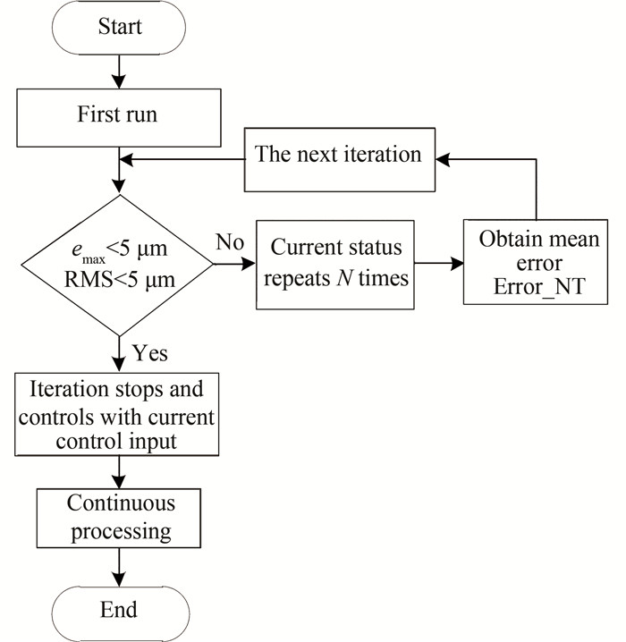
The experiment only used the feedback control. The actual position returned by the encoder was collected, the tracking error of each operation was calculated and then repeated multiple times (e.g., 100 times), and the average errormean NT was obtained. The average was used as the input for the iterative learning error because it is the average value, which is a filtering of the error signal. When the amount of running times was large enough, the irrational part was removed and the error input was softened, which can reduce the impact of accidental errors in the system. This is an essential approach during the experimental phase since some noise was introduced into the encoder feedback, which can accumulate as iterations progressively affect the normal operation of the system. Running the system for multiple times in the same state can also reveal the stability of the iterative learning control in the state of constant iterative compensation, which indicates that it is practically feasible to turn off the iterative control as appropriate. The mechanism is shown in Fig. 32.
|
Fig.32 Flow chart of ladder iterative learning mechanism |
First of all, repeat trials for several times without iterations, then get the errors and the average errors from computation. After the iteration, the method was continued until the amount of iteration control was closed to the desired control amount, the error dropped to the desired range, and the iterative mechanism could be chosen to close.
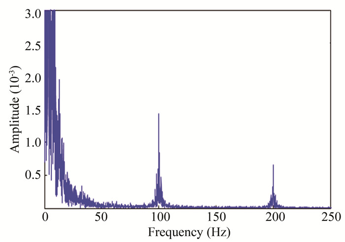
By comparing Fig. 33 and Fig. 34, the mean of multiple errors was obtained, which was also equivalent to a certain filtering and could make the error signal flatter. Some high-frequency signals in a certain error were attenuated in errormean, which proved that "ladder-type iterative learning" is necessary. Likewise, for each iteration, repeat the current state, run the same number of times, and then find the average errormean, followed by the operation. At the same time, adjust the learning gain according to the changes of each error.
|
Fig.33 Frequency-amplitude plot for the first error |

|
Fig.34 Errormean frequency-amplitude |
If the error attenuates too slowly, the learning gain and the rate of error convergence increase, which will converge to an acceptable level. With this method, the chances that errors impact the overall iterative process can be reduced, and the tasks to converge to the desired range can be completed with attempts.
6.3 Open-Loop Iterative Learning ExperimentWith the aforementioned butterfly trajectory, by using an open-loop P-type iterative learning, the variation of RMSE after several iterations is demonstrated in Fig. 35.

|
Fig.35 Variation of RMSE during different runs |
It can be seen from Fig. 35 that the RMSE of the system monotonously decayed, and after the fourth operation, it decreased to less than 0.01 mm, reflecting the validity of the iterative mechanism.
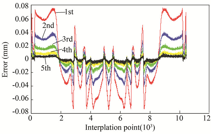
The overall error contrast is shown in Fig. 36, in which the first time is a simple feedback control, and the maximum overall error was about 0.070 mm. For the second run, the maximum overall error was about 0.040 mm, and the maximum overall run-time error was about 0.020 mm. The maximum run-time error was about 0.015 mm and the maximum run-in error was about 0.010 mm for the fifth run. It clearly shows the effect of iteration on the accuracy of the lift compared with the simple feedback control.
|
Fig.36 Run-time error curve |
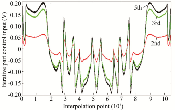
The iterative learning control was used to optimize and adjust the control variables. Fig. 37 demonstrates the changes of iterative control variables with the iterative operation. Since the initial running only had feedback control, the control of the iterative part started from the second runtime, and from the second to the fifth run, the control of the iterative part grew rapidly and gradually became "dominant".
|
Fig.37 Control curves of the iterative part in different runs |
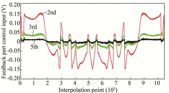
Fig. 38 shows the variation of the control quantity of the feedback part with iterative operation. From the second run to the fifth run, the control part of the feedback part decayed gradually, and the proportion of the control part became smaller and smaller.
|
Fig.38 Curve of feedback control during different times of operation |
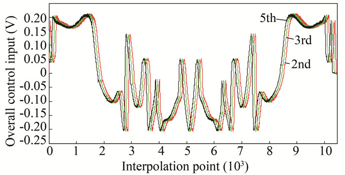
The change of the overall control volume is shown in Fig. 39. After the input trajectory speed planning was completed, the corresponding expected control volume could be deduced and is a constant value. Sum of the control part of the iterative part and the control part of the feedback part remained the same, but the two parts were "extroverted", i.e., as the iteration proceeded, the control amount of the iterative part became larger, which played an increasingly greater role, whereas that of the feedback part became smaller, being less important, and finally played a role to ensure system stability and interference suppression. By analyzing the changes of control volume, the essence of iteration became clearer.
|
Fig.39 Change curve of the overall control in different runs |
Due to the high frequency noise, the RMSE increased with iteration, which can be avoided with the following two measures:
1) Use the method of "switching iterative learning". Through judging the maximum tracking error and the RMSE, when they converge to the appropriate range, stop the iterative learning, and then the iterative learning control volume obtained at this time is saved as a constant compensation. However, when the system tracking error does not enter the allowable range of error and begins to increase, the method is not applicable and the second measure should be adopted;
2) Use the method of off-line low-pass filter. With the help of open-loop iterative structure, the off-line low-pass filter can be applied to filter out the high-frequency noise caused by the divergence error.
Since the open-loop iterative learning is the superimposition of control quantity in current time and the error in last time as the feedforward compensation part of this time, when the error dropped to a reasonable range, the part of each feedforward control part of the amount was constant, so the system would continue in its current state, and high-frequency noise would not be introduced, leading to system divergence.
However, when the error does not drop to the ideal range and begins to sharply increase, the processing effect cannot be achieved and should be combined with the off-line low-pass filter.
Based on the aforementioned method, the zero-phase off-line filtering was introduced to perform low-pass filtering on the zero-clearing gap after the running of the system. For the open-loop iterative learning structure, the method is suitable for filtering after the end of the second run at the corresponding interpolation point to fill the system. With iteration, high-frequency noise no longer accumulated and the error became monotonously convergent. When the error falls into the allowable range, the feedback control of the controller becomes very small, and the feedforward control quantity occupies most of the control input, during which the error will no longer be infinitely reduced with limitations of the servo system hardware. At this point, the iteration mechanism can be turned off, and the current control volume is stored as a constant control compensation added to the system. The result of this method is presented in Fig. 40, which proves that the method can be applied when faced with the same trajectory, reflecting the "memory" function of iterative learning.

|
Fig.40 Switch-type iterative learning RMSE curve |
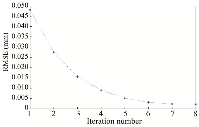
In Fig. 41, after the introduction of off-line low-pass filter, RMSE of the system operation showed a monotone decay trend. The algorithm effectively solved the problem of partial divergence error in iterative operation.
|
Fig.41 RMSE curve of filter-based iterative learning control |
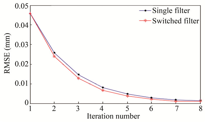
Using the switchable filter (Fig. 42), the RMSE of the system also tended to monotonously decay and was improved on the original basis. Especially in previous iterations, the RMSE of the same iteration was different.
|
Fig.42 Variation of RMSE with different filters |
7 Conclusions
Simulation and experiment were conducted with the combination of control layer and theoretical analysis, and the design and application of the iterative learning controller problems were discussed. In the existing numerical control system, the iterative mechanism was not joined. To further improve the precision and efficiency of single-piece high-volume machining, this paper elaborates the concrete problems of iterative learning application, and the main achievements are as follows:
1) The actual trajectory in machining was analyzed. For simple trajectory, only the feedback control with superposition velocity feedforward can achieve better control effect. For complex trajectory control, it is difficult to achieve a satisfactory result through feedback control of superposition velocity, so the iterative learning control and the open-loop iterative learning controller were designed. The expected control quantity was analyzed, and the iteration mechanism could be closed when the control quantity of the iterative part approached the expected control quantity. The idea of "ladder-type iteration" was proposed, which can preliminarily realize the effect of filtering, average the multiple repetitive errors, and filter out some of the high-frequency noise errors. Meanwhile, simulation was used to demonstrate the inhibitory effect of iterative learning on repetitive interference.
2) A design of filter-type iterative learning method was proposed, which solved the problem of error divergence in the process of iterative learning. Design of the corresponding low-pass filter was introduced and the result was verified. In order to further improve the accuracy of the convergence, time-frequency analysis of complex trajectory input was performed. According to the input characteristics, filters with different cutoff-frequencies were used in different time periods during operation to switch the cutoff-frequency filter, and the effectiveness was verified by simulation results, in which the maximum error within the convergence was 0.01 mm.
To sum up, this paper implements the design of a filter-based open-loop iterative learning controller on a TIMAX machine tool. However, there is still a need to further study the optimization of the experiment, in which a fixed gain, for different complex trajectories, should be combined with its speed, acceleration characteristics, and sub-segment. The use of adaptive gain learning algorithm can reach the control target efficiently.
| [1] |
Uchiyama M. Formation of high-speed motion pattern of a mechanical arm by trial. Transactions of the Society of Instrument and Control Engineers, 1978, 14(6): 706-712. DOI:10.9746/sicetr1965.14.706 (  0) 0) |
| [2] |
Arimoto S, Kawamura S, Miyazaki F. Bettering operation of robots by learning. Journal of Robotic Systems, 1984, 1(6): 123-140. DOI:10.1002/rob.4620010203 (  0) 0) |
| [3] |
Zhou W, Yu M, Huang D Q. A high-order internal model based iterative learning control scheme for discrete linear time-varying systems. International Journal of Automation and Computing, 2015, 12(3): 330-336. DOI:10.1007/s11633-015-0886-x (  0) 0) |
| [4] |
Chen Y, Gong Z, Wen C. Analysis of a high-order iterative learning control algorithm for uncertain nonlinear systems with state delays. Automatica, 1998, 34(6): 345-353. DOI:10.1016/S0005-1098(97)00196-9 (  0) 0) |
| [5] |
Li H S. Higher-order iterative learning control of non-linear system with disturbance. Pattern Recognition and Artificial Intelligence, 2006, 19(4): 450-454. (in Chinese) (  0) 0) |
| [6] |
Bien Z, Xu J X. Iterative learning control: analysis, design, integration and application. Norwell, MA, USA: Kluwer Academic Publishers, 1998, 65-77. (  0) 0) |
| [7] |
Longman R W. Iterative learning control and repetitive control for engineering practice. International Journal of Control, 2000, 73(10): 930-954. DOI:10.1080/002071700405905 (  0) 0) |
| [8] |
Longman R W, Huang Y C. The phenomenon of apparent convergence followed by divergence in learning and repetitive control. Intelligent Automation & Soft Computing, 2002, 8(2): 107-128. DOI:10.1080/10798587.2002.10644210 (  0) 0) |
| [9] |
Elci H, Longman R W, Phan M, et al. Discrete frequency based learning control for precision motion control. Proceedings of IEEE International Conference on Systems, Man, and Cybernetics. Piscataway: IEEE, 1994, 2967-2773. DOI:10.1109/ICSMC.1994.400292 (  0) 0) |
| [10] |
Shi Y, Longman R W. The influence on stability robustness of compromising on the zero tracking error requirement in repetitive control. The Journal of the Astronautical Sciences, 2012, 59(1-2): 441-458. DOI:10.1007/s40295-013-0027-8 (  0) 0) |
| [11] |
Li C, Wang F L, Dong Z R, et al. Injection velocity control in injection molding by iterative learning control with zero-phase filtering. Information and Control, 2009, 38(3): 293-296. (in Chinese) (  0) 0) |
| [12] |
Tsai M S, Yen C L, Yau H T. Integration of an empirical mode decomposition algorithm with iterative learning control for high-precision machining. IEEE/ASME Transactions on Mechatronics, 2013, 18(3): 878-886. DOI:10.1109/TMECH.2012.2194162 (  0) 0) |
| [13] |
Huang N E, Shen Z, Long S R, et al. The empirical mode decomposition and the Hilbert spectrum for nonlinear and non-stationary time series analysis. The Royal Society, 1998, 454(1971): 903-995. DOI:10.1098/rspa.1998.0193 (  0) 0) |
| [14] |
Elci H, Longman R W, Phan M Q, et al. Simple learning control made practical by zero-phase filtering: applications to robotics. IEEE Transactions on Circuits and Systems I: Fundamental Theory and Applications, 2002, 49(6): 753-767. DOI:10.1109/TCSI.2002.1010031 (  0) 0) |
| [15] |
Zhang B, Wang D, Ye Y. Cutoff-frequency phase-in iterative learning control. IEEE Transactions on Control Systems Technology, 2009, 17(3): 681-687. DOI:10.1109/TCST.2008.2000986 (  0) 0) |
| [16] |
Rotariu I, Steinbuch M, Ellenbroek R. Adaptive iterative learning control for high precision motion systems. IEEE Transactions on Control Systems Technology, 2008, 16(5): 1075-1082. DOI:10.1109/TCST.2007.906319 (  0) 0) |
| [17] |
Huang C E, Chen J S. Control of a pneumatic power active lower-limb orthosis with filter-based iterative learning control. International Journal of Systems Science, 2014, 45(5): 915-934. DOI:10.1080/00207721.2012.743052 (  0) 0) |
| [18] |
Bristow D, Tharayil M, Alleyne A G. A survey of iterative learning control. IEEE Control Systems Magazine, 2006, 26(3): 96-114. DOI:10.1109/MCS.2006.1636313 (  0) 0) |
 2020, Vol. 75


