Structural topology optimization (STO) focuses on determining the optimal layout of material inside the given design domain. As an optimization problem, it has one or more objective functions such as compliance, weight, and frequency, which subject to some constraints like volume, stress, and displacement. The material distribution is described by the density variable with value 0 or 1 at each point in the design domain. Considering the difficulty of solving the problem directly, the design domain is typically discretized into a large number of finite elements, so the nodal or element-wise densities can be used as the solution. Moreover, the densities are set as continuous variables varying from 0 to 1, thus the gradient becomes available.
As a continuous density-based method, solid isotropic material with penalization (SIMP), originally developed by Bendsøe[1], Zhou and Rozvany[2-3], is the most popular methodology for STO, which can be solved by some gradient-based optimization algorithms efficiently, such as optimal criteria (OC) and the method of moving asymptotes (MMA).
Instead of using continuous density variables, bi-directional evolutionary structural optimization (BESO), developed by Young et al.[4] and Huang and Xie[5], directly removes the elements with low sensitivity and adds the elements with high sensitivity step by step. Although using gradient for updating the discrete variables will generate error to some extent, BESO is comparable to SIMP in the quality of solutions and the computational efficiency for a large number of problems. Furthermore, because of its discrete formulation, it is more convenient to combine BESO with other algorithms.
1.2 Intelligence Algorithms in STODue to the material penalization, neither SIMP[6]nor BESO[7] can guarantee the convergence to a global optimum. A possible approach to overcome the difficulty is to introduce the global search techniques, such as heuristic algorithms like Genetic Algorithms[8-9] (GA), Ant Colonies[10-11], and Particle Swarms[12]. But even global search techniques cannot guarantee the convergence to the global optima for STO problems, and some non-gradient approaches show an extremely low computational efficiency[13] because of the astronomical number of the combinations of design variables. Thus, combining the advantages of gradient information and global search strategies is a compromising way to get an optimized solution. For example, GESO[8] is a successful combination of GA and ESO, in which the sensitivities calculated by BESO is used to keep the solving process effective and convergent, and GA operators are applied to improve the global search ability. Furthermore, Zuo et al.[9] combined GA with BESO to help recover those important elements, which is an improvement of GESO.
Over the past few years, considerable attention has been paid to STO problems by machine learning algorithms. For those problems whose sensitivity information of the design variables is difficult to calculate or even not available, Aulig and Olhofer[14-15] utilized some machine learning algorithms like linear regression, support vector machine, and neural network to replace the process of calculating the sensitivity. As for deep learning, convolutional neural network (CNN) and generative adversarial network (GAN) are used for generating the final structure with negligible computational time by inputting the intermediate results or even initial conditions[16-19]. However, this end-to-end learning method can only figure out problems similar to the training samples, which limits the scope of its applicability.
Reinforcement learning (RL) is another branch of machine learning, which learns how to get the maximum reward in the environment by trial and error constantly. In contrast to supervised learning, reinforcement learning may be less efficient but has the potential to explore unseen problems and gain better results beyond the history of human experience. Unfortunately, reinforcement learning has not yet been used to solve STO problems directly. The reason may lie in the enormous number of design variables. After all, reinforcement learning has recently been used for solving combinatorial optimization problems such as the traveling salesman problem with up to only 100 nodes and the 0-1 KnapSack problem with up to only 200 nodes[20], in which the number of the combinations of variables is much less than the problem faced in topology optimization, so RL needs to be proceeded with the help of prior knowledge.
1.3 Generative DesignGenerative design is the process of exploring the variants of a design beyond only one design traditionally[21]. Simple exploration methods are varying geometrical parameters[22] or problem definitions[23], whose search ability is limited. More complex exploration methods are achieved using deep neural networks such as CNN and GAN[14-18, 24]. The search scope is indeed enlarged in this way, but the drawbacks are the excessive computing source to prepare the training data and some methods are lack of mechanical analysis to guarantee the engineering performance.
1.4 Research PurposeIn this paper, a method combining BESO with RL for generative design is proposed. Each element was considered as an agent, whose value function was updated by Monte-Carlo reinforcement learning based on its sensitivity, which could make use of the previous experience to achieve better results. Also, ε-greedy policy was used in the procedure of adding and deleting elements in order to introduce the uncertainty, so that the search ability could be improved. Finally, a group of different quasi-optimal solutions with acceptable compliance were generated for designers.
The remainder of this paper is organized as follows. Section 2 provides an introduction of the corresponding reinforcement learning techniques. Section 3 describes our proposed method that combines BESO with RL in detail. The results of several well-known 2D and 3D minimum compliance problems are given as validations in Section 4. Finally, Section 5 draws the conclusion.
2 Reinforcement Learning 2.1 Brief IntroductionReinforcement learning has three key elements: state s, action a, and reward r. The process of learning can be described as the interaction between the agent and the environment. The agent chooses action at based on the current state st, then the environment responds to these actions and acquaints the agent with the reward rt+1 as well as the next state st+1. Finally, the policy π, which consists of a series of actions, is learned to maximize the cumulative reward in the future. Sometimes the agent would rather sacrifice the short-term reward in order to get more long-term reward. Thus, reinforcement learning is adaptive for solving sequential decision problems.
When selecting the actions, there are two different kinds of methods: policy-based method and value-based method. The former determines the policy directly, while the latter determines the policy implicitly by value function, which are used in this paper for its convenience to express the importance of elements.
2.2 First-visit Monte-Carlo Reinforcement LearningIn this paper, first-visit Monte-Carlo method, which has been widely studied since the 1940s[25], is used to evaluate the value function V. The information in episodes under policy π can be represented as a sequence:
| $ {s_1},{a_1},{r_2},{s_2},{a_2}, \cdots ,{s_t},{a_t},{r_{t + 1}}, \cdots ,{s_k} \backsim {\rm{ \mathsf{ π} }} $ |
Gt is the return of the state st, which is calculated as the total discounted reward that follows the first occurrence of st:
| $ \begin{array}{l} {G_t} = {r_{t + 1}} + \gamma V({s_{t + 1}}) = {r_{t + 1}} + \gamma {r_{t + 2}} + \\ {\kern 1pt} {\kern 1pt} {\kern 1pt} {\kern 1pt} {\kern 1pt} {\kern 1pt} {\kern 1pt} {\kern 1pt} {\kern 1pt} {\kern 1pt} {\kern 1pt} {\kern 1pt} {\kern 1pt} {\kern 1pt} {\kern 1pt} \cdots \cdots + {\gamma ^{T - 1}}{r_T} \end{array} $ | (1) |
where T denotes the terminal time, and the discount factor γ is in the range of 0 to 1. Then, the value function V(s) of a state s is calculated as the expected return in the future:
| $ V(s) = E[{G_t}|{s_t} = s] $ | (2) |
There are two other calculation methods for calculating the value function, namely dynamic programming and temporal-difference learning, which are not suitable for STO because abundant iterations are needed.
2.3 ε-greedy PolicyExploration-exploitation dilemma is a fundamental problem of RL. Exploitation means making the best decision based on current information, while exploration indicates gathering more information, which helps to make the best overall decision at the expense of the efficiency.
ε-greedy policy is a common method for exploration and mostly used for discrete action spaces in RL, which is defined as[25]:
| $ {\rm{ \mathsf{ π} }}(a|s) \leftarrow \left\{ {\begin{array}{*{20}{l}} {1 - \varepsilon + \frac{\varepsilon }{{\left| {A(\varepsilon )} \right|}},}&{{\rm{if}}{\kern 1pt} {\kern 1pt} a = {a^*}}\\ {\frac{\varepsilon }{{|A(\varepsilon )|}},}&{{\rm{if}}{\kern 1pt} {\kern 1pt} a \ne {a^*}} \end{array}} \right. $ | (3) |
where a* denotes the best action for maximizing the value function, and |A(s)| is the total number of actions in the state. By choosing an appropriate value of ε, the balance between exploration and exploitation can be well controlled. In general, a decay schedule for ε is usually added to reach the convergence.
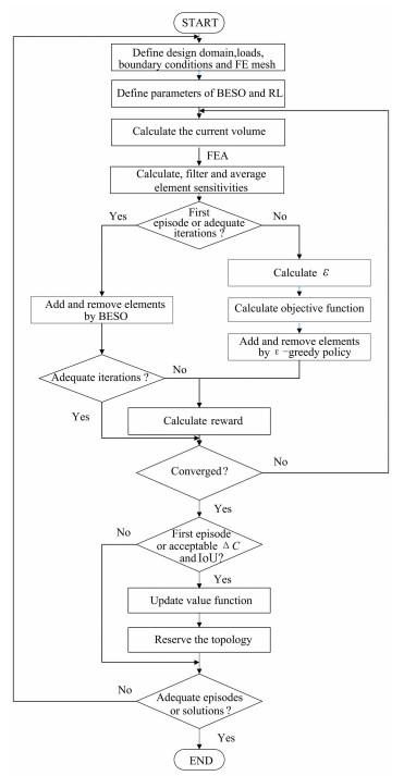
3 Continuum STO Using RL and BESOIn this section, a new method combining BESO with RL for continuum topology optimization problem of minimum compliance is proposed and described. The flowchart of the proposed method is shown in Fig. 1.
|
Fig.1 Flowchart of the combined method |
BESO method was utilized in the first episode to provide prior knowledge to create a good benchmark for evaluation and guarantee a stable value function, so as to avoid the inefficiency of searching from scratch. Then during the subsequent episodes, the problem was solved repeatedly, the value functions were updated simultaneously, and elements were removed and added based on their objective functions by ε-greedy policy. The final structure of each episode was reserved in the quasi-optimal solution set unless it satisfied the two metrics about the compliance and diversity. In the rest of the section, the procedure is explained in detail.
3.1 Problem StatementsAs the most typical topology optimization problem, minimum compliance STO under a certain limit of volume based on the density-based method is defined as
| $ \begin{array}{l} {\rm{Min}}:\mathit{\boldsymbol{C}} = \frac{1}{2}{\mathit{\boldsymbol{f}}^{\bf{T}}}\mathit{\boldsymbol{u}}\\ {\rm{Subject}}{\kern 1pt} {\kern 1pt} {\rm{to}}:{\rm{Vo}}{{\rm{l}}^*} - \sum\limits_e^N {{\rm{Vo}}{{\rm{l}}_e}} {\kern 1pt} {x_e},{x_e} = {x_{{\rm{min}}}}{\kern 1pt} {\rm{or}}{\kern 1pt} {\kern 1pt} 1 \end{array} $ | (4) |
where C is the structure compliance, which is also called the strain energy. u is the displacement vector, force vector f=Ku. Global stiffness matrix
In BESO, the sensitivity of a solid element is equal to the change of the compliance of the structure when this element is removed[27], and the sensitivities for void elements are zero, as in[7]
| $ {\alpha _e} = \left\{ {\begin{array}{*{20}{l}} {\frac{1}{2}p{\kern 1pt} x_e^{p - 1}\mathit{\boldsymbol{u}}_e^{\rm{T}}{\mathit{\boldsymbol{K}}_e}{\mathit{\boldsymbol{u}}_e},}&{{\rm{when}}{\kern 1pt} {\kern 1pt} {x_e} = 1}\\ {0,}&{{\rm{when}}{\kern 1pt} {\kern 1pt} {x_e} = {x_{{\rm{min}}}}} \end{array}} \right. $ | (5) |
where ue is the nodal displacement vector of the ith element, and Ke is the element stiffness matrix.
The filter scheme is achieved by averaging the elemental sensitivities:
| $ {\alpha _e} = \frac{{\sum\limits_{j = 1}^N {{H_{ej}}} {\alpha _j}}}{{\sum\limits_{j = 1}^N {{H_{ej}}} }} $ | (6) |
where the weight factor Hej is calculated by:
| $ {H_{ej}} = {r_{{\rm{min}}}} - {r_{ej}},{\kern 1pt} {\kern 1pt} {\kern 1pt} {\kern 1pt} \{ e{\kern 1pt} {\kern 1pt} {\kern 1pt} {\kern 1pt} \in {\kern 1pt} {\kern 1pt} {\kern 1pt} {\kern 1pt} N|{\kern 1pt} {\kern 1pt} {\kern 1pt} {r_{ej}}\} $ | (7) |
in which rej means the distance between the center of the eth and the jth element, rmin is the filter radius.
Furthermore, the element sensitivities should be changed into the mean value of the sensitivities of the current iteration and the last iteration[28]:
| $ {\alpha _e} = \frac{{\alpha _e^t + \alpha _e^{t - 1}}}{2} $ | (8) |
where t denotes the current iteration number. It is a simple but effective way to keep the solving process more stable and easier to converge.
3.3 Value Function ApproximationThe STO problem belongs to a 0-1 integer planning problem, and the solving process is a kind of sequential decision process which can be represented by a policy π, so the policy π can be acquired by RL. But it should be noted that if the whole structure is viewed as an agent, the number of the combination of actions reaches up to over 1085 just for a simple problem like designing a cantilever beam discretized by 288 elements and within a 50% volume fraction constraint[13]. Due to the complexity, elements were treated as individuals.
The features of the reinforcement learning algorithm are defined below. The state was defined as the current iteration number in each episode, which was sequential, and each state appeared once and only once during one episode. Moreover, it is noted that the volume fraction of the structure was fixed for each state. The action was the addition or removal of the element, and the reward was characterized by the updated density of elements:
| $ r_e^t = \left\{ {\begin{array}{*{20}{l}} {1,}&{{\rm{if}}{\kern 1pt} {\kern 1pt} {x^{t + 1}} = 1}\\ {0,}&{{\rm{if}}{\kern 1pt} {\kern 1pt} x_e^{t + 1} = {x_{{\rm{min}}}}} \end{array}} \right. $ | (9) |
As each state was visited only once during one episode, the first-visit Monte-Carlo RL method exactly satisfied the requirement. The return Get was calculated according to Eq.(1), and a weight was added to Get when the value function was approximated:
| $ V_e^\pi (s) = E_e^\pi \left[ {(2 - \frac{C}{{{C_B}}})G_e^t|{s_t} = s} \right] $ | (10) |
where C denotes the compliance of the final structure and CB is the compliance of the final structure generated by BESO as a benchmark. In this way, the policy of the final structure with lower compliance had more influence on the value function and vice versa, then the search was guided to the direction closer to the optimum.
During the solving process of BESO, the changes in earlier iterations had a crucial impact on the determination of the final structure, when the volume fraction declined close to the minimum, the structure varied little, because there were not so many elements removed or added in each iteration. Hence, exploring in the latter iterations seemed valueless and would prolong the time for convergence. As a result, a decision was made to end up updating the value function after 5 iterations when volume fractions were invariant, so as to keep the balance between exploration and efficiency. The remaining work was to be accomplished by BESO until convergence.
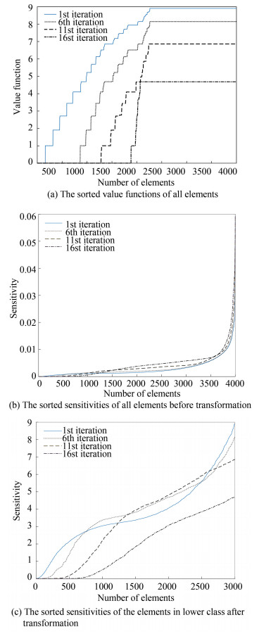
3.4 Removal and AdditionAccording to the criterion that the elements are sorted by, the objective function F is the weighted sum of the value function V and the current sensitivity α. The numerical distributions of V and α can be seen in Fig. 2(a) and 2(b), respectively, which derive from several intermediate results of a case. In order to make V and α equal in the order of magnitude, a linear transformation similar to min-max normalization was applied to α according to the distribution of V.
|
Fig.2 Distribution of value functions and sensitivities of several intermediate results of a case |
The elements were divided into two classes based on the ranking of α. The proportion of elements ranked in the higher class was set as
| $ {P_{{\rm{higher}}}} = {\rm{Vo}}{{\rm{l}}^*}/2 $ | (11) |
where Vol* is the volume fraction constraint. Elements of the higher class could not be removed considering that the whole structure may collapse suddenly. So it should be guaranteed that the values of α were roughly equal to the values of V for the lower class (Fig. 2(c)). α was transformed as
| $ \begin{array}{l} {\alpha ^e}(s) \leftarrow {[V_e^\pi (s)]_{{\rm{min}}}} + ({[V_e^\pi (s)]_{{\rm{max}}}} - {[V_e^\pi (s)]_{{\rm{min}}}}) \cdot \\ {\kern 1pt} {\kern 1pt} {\kern 1pt} {\kern 1pt} {\kern 1pt} {\kern 1pt} {\kern 1pt} {\kern 1pt} {\kern 1pt} {\kern 1pt} {\kern 1pt} {\kern 1pt} {\kern 1pt} {\kern 1pt} {\kern 1pt} {\kern 1pt} {\kern 1pt} {\kern 1pt} {\kern 1pt} {\kern 1pt} {\kern 1pt} {\kern 1pt} {\kern 1pt} {\kern 1pt} {\kern 1pt} {\kern 1pt} {\kern 1pt} {\kern 1pt} {\kern 1pt} {\kern 1pt} {\kern 1pt} {\kern 1pt} {\kern 1pt} {\kern 1pt} {\kern 1pt} {\kern 1pt} {\kern 1pt} {\kern 1pt} {\kern 1pt} {\kern 1pt} {\kern 1pt} {\kern 1pt} {\kern 1pt} \frac{{{\alpha ^e}(s) - {{[{\alpha ^e}(s)]}_{{\rm{min}}}}}}{{{{[\alpha _{{\rm{lower}}}^e(s)]}_{{\rm{max}}}} - {{[{\alpha ^e}(s)]}_{{\rm{min}}}}}} \end{array} $ | (12) |
Then, the objective function F is calculated as
| $ {F^e}(s) = \omega V_\pi ^e(s) + (1 - \omega ){\alpha ^e}(s) $ | (13) |
where ω is a weight that controls the search scope to keep the convergence. ω has a strong influence on the ranking of the elements as shown in the jagged curve of Fig. 2(a). Thus generally, ω is a small value varying from 0.005 to 0.01 for common simple 2D cases, and a bigger ω is suitable for 3D cases with more design variables and lower volume fraction constraint.
ε-greedy policy was used to decide whether an element should be added or removed. In BESO, elements were deleted depending on the sensitivities completely like the greedy algorithm. In ε-greedy policy, after sorting the elements by their objective functions, the elements were divided into higher class and lower class, and the bottom (1-ε) fraction of the elements to be removed in this iteration were firstly deleted in the same way as BESO, while the other ε fraction were deleted randomly from the rest in the lower class.
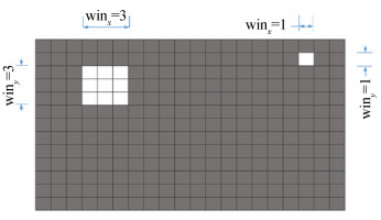
To enhance the effectiveness of the random search, a 'search window' as shown in Fig. 3 was used to change the scope of removal. For 2D problems, the search window has two parameters: winx and winy, representing the scope of the adjacent elements in x and y direction to be deleted together when an element is removed. A larger winx or winy is recommended to be used on a denser mesh. For 3D problems, a three-dimensional search window is needed with an additional parameter winz.
|
Fig.3 Search windows of different sizes |
Like the penalization mechanism of GA operators[9], in each iteration, ε declined gradually to obtain a convergent solution, and the scheme was formed as follows:
| $ \varepsilon \leftarrow {\varepsilon _0} - {\varepsilon _0}{(t/{t_0})^3} $ | (14) |
where ε0 denotes the ε at the beginning, and t0 means the number of iterations when the volume fraction just reaches the minimum.
3.5 Convergence CriterionThe convergence criterion used in the combined method is the same as BESO[28]. In one episode, the update of topology will not be stopped unless the volume constraint Vol* is reached and the following criterion is satisfied:
| $ \frac{{|\sum\limits_{i = 1}^I {({C_{t - i + 1}} - {C_{t - N - i + 1}})} |}}{{\sum\limits_{i = 1}^1 {{C_{t - i + 1}}} }} \le \tau $ | (15) |
where I denotes an integral number which was set to 5 in this study, τ represents the convergence tolerance and is always a specified small value.
3.6 Evaluation of Final StructuresTo get a group of quasi-optimal solutions with low compliance as well as enough novelty, two metrics were used to evaluate the performance of the final structure in each episode:
First, the difference of compliance between the final structure and the benchmark was considered:
| $ \Delta C = (C - {C_B})/{C_B} $ | (16) |
Only the results with ΔC less than 0.2 were acceptable in this study.
Another metric Intersection-over-Union (IoU), which is a common evaluation metric for the similarity of images in the field of object detection, was calculated as the ratio of the intersection to the union of two rectangles named candidate bound CB and ground truth bound GB:
| $ {\rm{IoU = }}\frac{{{\rm{ area (CB)}} \cap {\rm{area (CB)}}}}{{{\rm{ area (CB)}} \cup {\rm{area (CB)}}}} $ | (17) |
In this study, the threshold was set to be 0.9, and IoU was also available in 3D, where 'area' in Eq. (17) should be replaced by "volume".
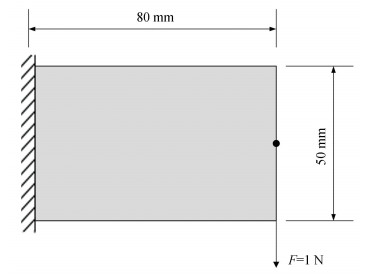
4 Results and Discussions 4.1 Cantilever BeamThe first example considered the stiffness optimization design of a cantilever beam, which was subjected to a concentrated force applied at the center of the free end as shown in Fig. 4. The length and height of the design domain was 80 mm and 50 mm, respectively, and it was discretized into 80×50 four-node quadrilateral elements. Material properties were Young's modulus E=1 MPa and Poisson's ratio υ=0.3. The objective volume fraction was set to be 50% of the design domain. Parameters of BESO are shown as follows: the evolution volume ratio ER=0.04, the maximum volume addition ratio, a filter radius rmin=4 mm, the minimum design variable xmin=0.001, the convergence criterion τ=0.1%, and the penalty exponent p=3.0. Moreover, parameters concerning RL are as follows: the discount factor γ=0.9, ε0=0.1, weight ω=0.005, and winx=winy=3. It is noted that the symmetry between the upper half and lower half of the beam was considered during removing and adding the elements.
|
Fig.4 Dimensions of the design domain of a cantilever beam with loading and boundary conditions |
The final topology of BESO is shown in Fig. 5(a), and eight quasi-optimal solutions of the combined method are displayed in Fig. 5(b)-5(i). Finally, the information about compliance, IoU, and iterations of the final result in each episode is given in Table 1. It can be seen that the quasi-optimal solutions are different from the result of BESO to various extent. Some are highly similar as shown in Fig. 5(f), and some change a lot as shown in Fig. 5(e) and 5(h), but their compliance is all within the scope of acceptability. Moreover, the structure in Fig. 5(f) even has less compliance than the referenced structure, which means the combined method indeed contributed to searching for global optimums. Furthermore, to get eight applicable solutions, 14 episodes were needed, and the difference in the number of iterations of each episode were not significant. All in all, the quasi-optimal solutions were generated within acceptable computation cost.

|
Fig.5 Final topologies of a cantilever beam by BESO method (a) and by combined method (b)-(k) |
| Table 1 Information of designs of a cantilever beam (Unsatisfactory metrics are deleted by strikethrough) |
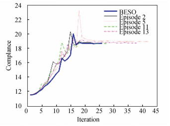
The evolutionary histories of the compliance are presented in Fig. 6. As can be observed, the compliance does not always increase as the number of iterations increases, and the evolution curve is usually not smooth. There are one or more peaks in each curve, and the amplitude and corresponding iteration of the peaks varies in different episodes, representing different search directions.
|
Fig.6 Evolutionary histories of the compliance for the cantilever |
It is worth noting that although increasing ω can help search for better results, it hampers diversity at the same time. For example, if ω is set to a relatively high value, such as 0.5, most solutions are with lower compliance than that of the benchmark, but also with extremely high IoU as shown in Table 2. It means that the solutions are lack of novelty and fail to provide designers with more information.
| Table 2 Information of designs of a cantilever beam (when ω=0.5, unsatisfactory metrics are deleted by strikethrough) |
4.2 L-shaped Beam
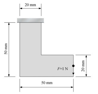
The second example demonstrates a design problem for an L-shaped beam as shown in Fig. 7, which was loaded at the center of the rightmost free end by F=-1 N.The beam was discretized into 1600 elements and the volume fraction was 40%. Material properties were E=1 MPa and υ=0.3. BESO parameters were set as ER=0.03, rmin=2 mm, xmin=0.001, τ=0.1%, and p=3.0. RL parameters were γ=0.9, ε0=0.1, ω=0.005, and winx=winy=1.
|
Fig.7 Design domain of an L-shaped beam with dimensions, boundary, and loading conditions |
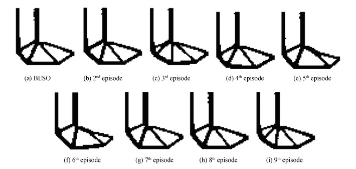
Final topologies obtained by BESO and the combined approach are shown in Fig. 8. The corresponding details are given in Table 3. All the eight results seem satisfactory, and half of them have lower compliance than the first generated by BESO method. It is noteworthy that an additional bar inside the structure as shown in Fig. 8(i) would help in decreasing the compliance. Another worthy information is that compared with a simpler design like example in Section 4.1, a more complicated structure is easier to satisfy the requirement of IoU.
|
Fig.8 Final topologies of the L-shaped beam by BESO method (a) and by combined method (b)-(k) |
| Table 3 Information of designs of an L-shaped beam |
4.3 3D Cantilever Beam
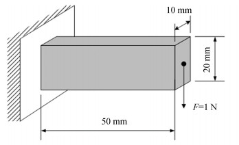
The proposed approach can be extended to three dimensions straightforwardly. An optimized design problem for a 3D cantilever beam is shown in Fig. 9. The design domain was divided into 50×20×10 and modeled using 10000 eight node cubic elements in total. The remaining volume fraction was only 10% volume of the design domain. Material with E=1 MPa and υ=0.3 was used. BESO parameters were ER=0.03, rmin=3 mm, xmin=0.001, τ=1% and p=3.0. Parameters relative to RL were generally similar to those of 2D problems, where γ=0.9, a lower ε0=0.05, a higher ω=0.01, and winx=winy=winz=1 for a 3D search window. The symmetry along y axis and z axis was considered.
|
Fig.9 Dimensions of the design domain with loading and boundary conditions for a 3D cantilever beam |
The optimal designs are shown in Fig. 10, and the corresponding information is in Table 4. As can be seen, the topologies in this 3D case vary in a greater degree compared with that in 2D cases despite more conservative parameters were chosen. As a cantilever beam, the IoU of the solutions of a three-dimensional beam is much lower than that in two dimensions, so the diversity of solution is easy to guarantee. However, divergence is more likely to occur in this case, for example, in the 9th episode. That is why a lower ε0 and a higher ω were selected to alleviate the problem.

|
Fig.10 Final topologies of the 3D cantilever beam by BESO method (a) and by combined method (b)-(k) |
| Table 4 Information of designs of a 3D cantilever beam(Unsatisfactory metrics are deleted by strikethrough) |
Table 5 shows the effect of main parameters ω and ε0. Six pairs of different parameters were chosen. In each case, the combined method was performed at most of the 21 episodes and was terminated early when 8 acceptable structures were obtained. The data in Table 5 was calculated by running the procedure for 10 times. It can be seen that decreasing ε0 can significantly avoid undesirable results, but the search scope is limited at the same time, so a balance between the convergence and the search ability should be kept by choosing an appropriate ε0. As ω changes from 0 to 0.1 (value function is not considered absolutely when ω=0), the number of solutions with an inacceptable C reduces gradually, which means the value function does help guarantee the quality of the solutions, but a too large ω is not recommended due to the decline in diversity.
| Table 5 Influence of main parameters on the performance of final designs |
4.4 Geometrically Nonlinear Cantilever Beam
The combined method was extended conveniently to geometrically nonlinear structures. In nonlinear analysis, complementary work and force control by Newton-Raphson method was used. The difference was that the complementary work WC should replace compliance as the final measurement:
| $ {\rm{Min}}:{W^C} = \mathop {\lim }\limits_{n \to \infty } [\frac{1}{2}\sum\limits_{i = 1}^n \Delta {\mathit{\boldsymbol{F}}^{\rm{T}}}({U_i} + {U_{i - 1}})] $ | (18) |
in which U means the displacement vector, ΔF is determined by the step used in Newton-Raphson method, i is the incremental number of the applied load, and n is the total number of increments.
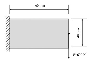
The stiffness optimization of a 2D cantilever beam is demonstrated considering the geometrical nonlinearity simultaneously. The structure with dimensions of 60 mm in length, 40 mm in width, and 10 mm in thickness is shown in Fig. 11. According to assumption, the available material only covers 50%. The material is linear elastic with E=1 GPa and υ=0.3. BESO parameters are ER=0.03, rmin=3 mm, xmin=0.001, τ=1%, and p=3.0. RL parameters are generally similar to those of 2D problems, where γ=0.9, a lower ε0=0.05, a higher ω=0.01, and a 3D search window with winx=winy=1. The symmetry constraint was no longer considered.
|
Fig.11 Dimensions of the design domain of a nonlinear cantilever beam with loading and boundary conditions |
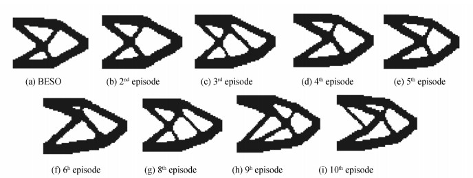
To judge which design was better, the complementary work WC was calculated by nonlinear FEM. The topologies as well as results are given in Table 6 and Fig. 12. Compared with the results of linear FEM in Section 4.1, most of the structures became less symmetric, which was caused not only by the randomness of the deletion but by the nonlinearity. As a result, the diversity of solution is easier to guarantee. In addition, the values of complementary work are still acceptable and not influenced too much by the asymmetry. As the computation cost used in nonlinear analysis becomes higher, more running time is needed, so optimizing large complex 3D nonlinear structures seems challengeable.
| Table 6 Information of designs of a nonlinear cantilever beam(Unsatisfactory metrics are deleted by strikethrough) |
|
Fig.12 Final topologies of the nonlinear cantilever beam by BESO method (a) and by combined method (b)-(k) |
5 Conclusions and Prospect
This paper presents a new approach for structural topology optimization combining the features of BESO method and reinforcement learning. During the process, the roles of BESO are providing the prior experience for RL and assisting in getting a convergent result in the final stage of each episode. As an auxiliary method to improve search ability, ε-greedy policy was utilized to disturb the search direction by deleting a fraction of elements randomly. In the meantime, the objective function consisting of the weighted sum of value function and sensitivity did well to help in getting convergent solutions with low compliance. The combined method was demonstrated on four compliance minimization problems of 2D and 3D, including one geometrically nonlinear problem. By fine-tuning the parameters like weight, ε, and the size of search window, a group of quasi-optimal solutions with acceptable engineering performance and novelty could be generated.
In contrast to traditional density-based approaches like SIMP and BESO which can only generate one determined solution and cannot guarantee the optimality, the proposed approach is able to create several different solutions with acceptable compliance. In theory, the structure with smallest value of compliance should be chosen as an optimum, but the one that fits the practical problem the most is the priority in practice. Thus, although some solutions proposed by this study are not better than that of BESO in compliance, they can serve as valuable alternatives for decision making in engineering.
For the combined method, the mechanical analysis needs restarting for each new episode, so the computing time in the following episodes is almost the same as that in the first episode. It has the potential to decrease the consumption by referring to similar information from previous episodes. Another improvement is hidden in the exploration methods. After all, ε-greedy policy is just a basic method. There are many other powerful approaches for exploration in RL.
Data availability
The corresponding code can be found at https://github.com/Nick0095/RL_BESO.
| [1] |
Bendsøe M P. Optimal shape design as a material distribution problem. Structural Optimization, 1989, 1: 193-202. DOI:10.1007/BF01650949 (  0) 0) |
| [2] |
Zhou M, Rozvany G I N. The coc algorithm. Part ii: Topological, geometry and generalised shape optimisation. Computer Methods in Applied Mechanics and Engineering, 1991, 89(1-3): 309-336. DOI:10.1016/0045-7825(91)90046-9 (  0) 0) |
| [3] |
Rozvany G I N, Zhou M, Birker T. Generalized shape optimization without homogenization. Structural Pptimization, 1992, 4(3-4): 250-252. DOI:10.1007/BF01742754 (  0) 0) |
| [4] |
Young V, Querin O M, Steven G P, et al. 3D and multiple load case bi-directional evolutionary structural optimization (BESO). Structural Optimization, 1999, 18(2-3): 183-192. DOI:10.1007/BF01195993 (  0) 0) |
| [5] |
Huang X, Xie Y M. Convergent and mesh-independent solutions for the bi-directional evolutionary structural optimization method. Finite Elements in Analysis and Design, 2007, 43(14): 1039-1049. DOI:10.1016/j.finel.2007.06.006 (  0) 0) |
| [6] |
Stolpe M, Svanberg K. On the trajectories of penalization methods for topology optimization. Structural and Multidisciplinary Optimization, 2001, 21: 128-139. DOI:10.1007/s001580050177 (  0) 0) |
| [7] |
Huang X, Zuo Z H, Xie Y M. Evolutionary topological optimization of vibrating continuum structures for natural frequencies. Computers & Structures, 2020, 88(5-6): 357-364. DOI:10.1016/j.compstruc.2009.11.011 (  0) 0) |
| [8] |
Liu X, Yi W J, Li Q S, et al. Genetic evolutionary structural optimization. Journal of Constructional Steel Research, 2008, 64(3): 305-311. DOI:10.1016/j.jcsr.2007.08.002 (  0) 0) |
| [9] |
Zuo Z H, Xie Y M, Huang X. Combining genetic algorithms with BESO for topology optimization. Structural and Multidisciplinary Optimization, 2009, 38: 511-523. DOI:10.1007/s00158-008-0297-5 (  0) 0) |
| [10] |
Kaveh A, Hassani B, Shojaee S, et al. Structural topology optimization using ant colony methodology. Engineering Structures, 2008, 30(9): 2559-2565. DOI:10.1016/j.engstruct.2008.02.012 (  0) 0) |
| [11] |
Luh G C, Lin C Y. Structural topology optimization using ant colony optimization algorithm. Applied Soft Computing, 2009, 9(4): 1343-1353. DOI:10.1016/j.asoc.2009.06.001 (  0) 0) |
| [12] |
Luh G C, Lin C Y, Lin Y S. A binary particle swarm optimization for continuum structural topology optimization. Applied Soft Computing, 2011, 11(2): 2833-2844. DOI:10.1016/j.asoc.2010.11.013 (  0) 0) |
| [13] |
Sigmund O. On the usefulness of non-gradient approaches in topology optimization. Structural and Multidisciplinary Optimization, 2011, 43(5): 589-596. DOI:10.1007/s00158-011-0638-7 (  0) 0) |
| [14] |
Aulig N, Olhofer M. Topology optimization by predicting sensitivities based on local state features. Proceedings of the 5th. European Conference on Computational Mechanics. Barcelona, Spain: WCCM XI-ECCM V-ECFD VI, 2014.
(  0) 0) |
| [15] |
Aulig N, Olhofer M. Neuro-evolutionary topology optimization of structures by utilizing local state features. Proceedings of the 2014 Annual Conference on Genetic and Evolutionary Computation. New York: ACM, 2014. 967-974. DOI: 10.1145/2576768.2598314.
(  0) 0) |
| [16] |
Sosnovik I, Oseledets I. Neural Networks for Topology Optimization. arXiv preprint arXiv: 1709.09578, 2019-12-23.
(  0) 0) |
| [17] |
Yu Y, Hur T, Jung J, et al. Deep learning for determining a near-optimal topological design without any iteration. Structural and Multidisciplinary Optimization, 2019, 59: 787-799. DOI:10.1007/s00158-018-2101-5 (  0) 0) |
| [18] |
Banga S, Gehani H, Bhilare S, et al. 3D Topology Optimization Using Convolutional Neural Networks, arXiv: 1808.07440, 2019-12-23.
(  0) 0) |
| [19] |
Rawat S, Shen M H H. Application of adversarial networks for 3D structural topology optimization. No. 2019-01-0829. SAE Technical Paper, 2019. DOI: 10.4271/2019-01-0829.
(  0) 0) |
| [20] |
Bello I, Pham H, Le Q V, et al. Neural Combinatorial Optimization with Reinforcement Learning. arXiv: 1611. 09940, 2019-12-23.
(  0) 0) |
| [21] |
McKnight M. Generative Design: What it is? How is it being used? Why it's a game changer. The International Conference on Design and Technology. Dubai: Knowledge E, 2017. 176-181. DOI: 10.18502/keg.v2i2.612.
(  0) 0) |
| [22] |
Matejka J, Glueck M, Bradner E, et al. Dream lens: Exploration and visualization of large-scale generative design datasets. Proceedings of the 2018 CHI Conference on Human Factors in Computing Systems. New York: ACM, 2018. DOI: 10.1145/3173574.3173943.
(  0) 0) |
| [23] |
Krish S. A practical generative design method. Computer-Aided Design, 2011, 43(1): 88-100. DOI:10.1016/j.cad.2010.09.009 (  0) 0) |
| [24] |
Oh S, Jung Y, Kim S, et al. Deep generative design: Integration of topology optimization and generative models. Journal of Mechanical Design, 2019, 141(11): 111405. DOI:10.1115/1.4044229 (  0) 0) |
| [25] |
Sutton R S, Barto A G. Reinforcement learning: An introduction. Massachusetts.MIT Press, 1998.19-114.
(  0) 0) |
| [26] |
Bendsøe M P, Sigmund O. Topology Optimization: Theory, Methods and Applications. Berlin: Springer-Verlag, 2003. 9-20.
(  0) 0) |
| [27] |
Chu D N, Xie Y M, Hira A, et al. Evolutionary structural optimization for problems with stiffness constraints. Finite Elements in Analysis and Design, 1996, 21(4): 239-251. DOI:10.1016/0168-874X(95)00043-S (  0) 0) |
| [28] |
Huang X H, Xie Y. Bi-directional evolutionary topology optimization for structures with geometrical and material nonlinearities. AIAA Journal, 2007, 45(1): 308-313. DOI:10.2514/1.25046 (  0) 0) |
 2021, Vol. 28


