2. State Key Laboratory of Disaster Reduction in Civil Engineering, Tongji University, Shanghai 200092, China;
3. School of Civil Engineering, Fujian University of Technology, Fuzhou 350118, China
In the wind-resistant design of structures, a common design process is to estimate wind-induced responses by equivalent static wind load (ESWL), which is a powerful tool for structural engineers to transform a complex dynamic calculation procedure into a simple static one. It has been adopted by most wind codes/standards of practice with respect to the wind design of structures in the world. ESWL can be defined as that the responses produced by the assumed static ESWLs are equal or approximate to the extreme responses produced by the actual dynamic wind loads. With ESWL obtained, structural engineers are able to evaluate the complex wind-induced dynamic responses using static analyses which they are familiar with. ESWL has become the bridge that connects wind engineers and practicing engineers, and plays an important role in civil engineering.
The concept of ESWL for a structure was initially proposed by wind engineering researchers when analyzing wind effects on tall buildings and high-rise structures. Later, the concept was introduced to estimate wind-induced dynamic responses of large-span roofs, long-span bridges, and so on. In the 1960s, Davenport firstly used random vibration theory to solve buffeting problems in wind engineering[1-2] and proposed the Gust Loading Factor (GLF) method[3] to calculate responses of tall buildings subject to wind. Davenport initially utilized displacement of tall buildings to calculate GLF and EWSLs. The GLF method proposed by Davenport is more appropriately called GLF method based on displacement. Later, other researchers developed this method and proposed GLF methods based on other responses such as base bending moment, shear force, and axial force. The ESWLs estimated by the GLF method are proportional to the mean wind load. Inertial Wind Load (IWL) method is another important ESWL estimation approach which directly adopts the inertial force induced by gust wind load to calculate ESWL[4-6]. The ESWL distribution estimated by IWL method is proportional to the inertial loads of the structure rather than the mean wind loads. IWL method has been adopted by the Chinese code of the Load Code for the Design of Building Structures[7] and is mainly used to calculate resonant ESWL. Besides, background is another crucial aspect of total response. For stiff structures, background dominates the wind-induced dynamic responses. Load-response correlation (LRC) method[8-11] is a critical approach to deal with background ESWL. LRC+IWL method[12-18] is a combination of LRC and IWL methods, which uses LRC method to handle the background ESWL and IWL method for the resonant part. With the two parts obtained, the total ESWLs can be acquired through an appropriate combination mode. Apart from the background and the resonant components, the coupled term between the two components are also considered in the total ESWL[19-20]. Universal ESWL (UESWL) is an important numerical estimation method that can simultaneously reproduce the largest responses in all subject members of a structure[21]. Blaise et al. proposed Principal Static Wind Loads (PSWL) method based on singular value decomposition technique to reconstruct the envelope of wind-induced structural responses in Gaussian[22] and non-Gaussian[23] contexts. In fact, UESWL distribution is a least-square approximation solution, but it is effective in many cases. Based on PSWLs, Patruno et al.[24-25] proposed an efficient approach to reconstruct envelope values of ESWLs of structures in a least square sense. In this approach, PSWLs are obtained through Proper Skin Modes[24] and an efficient gradient based optimization algorithm is used to replace Monte Carlo or evolutive optimization techniques.
GLF, IWL, LRC, LRC+IWL, UESWL, and PSWL are the main methods to estimate ESWL, among which the LRC method is a milestone in the research of ESWL[17]. The LRC method was firstly proposed by Kasperski and Niemann[8] when studying wind-induced responses of low-rise buildings and is regarded as an accurate method to estimate the background ESWL of a structure. According to the relationship between load and response, ESWL estimated by LRC method can be expressed by load-response correlation coefficients, RMS values of the fluctuating wind load, and peak factor. The derivation of the classical expression of LRC method is based on a specific response at a critical positon, and the corresponding ESWL distribution is unique. The Australian/New Zealand Standard AS/NZS 1170.2-Wind actions [26] and the ISO 4354-Wind Actions on Structures[27] adopt the LRC method in wind resistant design of structures. In addition, Dong et al.[28] proposed a multi-target ESWL method based on LRC method and proper orthogonal decomposition technique.
In this paper, a general expression of LRC method is derived. Based on the finite element model and a specific command response of a structure, the general expression of the LRC method is obtained by load-response correlation coefficients, RMS values of the fluctuating wind loads, response-response correlation coefficients, and peak factor in the form of matrices. In addition to the load-response correlation coefficients, the general expression also contains response-response correlation coefficients which extend the scope of the LRC method and reveal the inherent relationship between ESWL distribution and response-response correlation coefficient. Unlike the classical expression, the general expression can provide more optional ESWL distributions by taking account of different response-response correlation coefficients. The derivation also reveals the fact that even for a specific response at a concerned position, the ESWL distribution has more than one form and the classical expression is only one form of the general one. The general expression provides more options to estimate ESWL and further insight into the LRC method. Finally, a cable-stayed bridge, a three span continuous girder bridge, and a suspension bridge are taken as examples to verify the correctness of the general expression of LRC method.
This paper focuses on the derivation of general expression of LRC method and verifies its correctness by examples, and hopefully the potential usages of the methods can be found by researchers in this field. Differences between the general expression and the classical expression of LRC method are illustrated through theoretical derivation and examples. However, the aim of the paper is not to compare which expression is better than another one. In fact, in most cases, the wind load obtained by classical expression is the best of all ESWL distributions provided by general expression of LRC method. Only in the cases of estimating multi-target ESWLs, the general expression may have some advantages. The advantages and disadvantages of the LRC method compared with other ESWL estimation methods are not in the scope of discussion in this research neither.
1 Derivation of the Classical Expression of LRC MethodIn this section, the derivation of the classical expression for LRC method is presented[8-11]. According to the relationship between load and response, for discrete finite element model of a structure, any specific response Ri(t) at the position of node i can be expressed by the influence function and the wind loads under quasi-static assumption, as follows:
| $ \boldsymbol{R}_{i}(t)=\bar{\boldsymbol{R}}_{i}+\hat{\boldsymbol{R}}_{i}(t)=\boldsymbol{I}_{i}^{\mathrm{T}} \bar{\boldsymbol{F}}+\boldsymbol{I}_{i}^{\mathrm{T}} \hat{\boldsymbol{F}} $ | (1) |
where Ri,
| $ \boldsymbol{I}_{i}=\left[\begin{array}{lll} I_{i}^{1} & \cdots & I_{i}^{N-\mathrm{node}} \end{array}\right]^{\mathrm{T}} $ |
| $ \bar{\boldsymbol{F}}=\left[\begin{array}{lll} \bar{F}_{1} & \cdots & \bar{F}_{N-\mathrm{node}} \end{array}\right]^{\mathrm{T}} $ |
| $ \hat{\boldsymbol{F}}=\left[\begin{array}{lll}\hat{F}_{1}(t) & \cdots & \hat{F}_{N-\mathrm{node}}(t) \end{array}\right]^{\mathrm{T}} $ |
where T denotes the transpose of the matrix.
The response induced by fluctuating wind loads can be expressed as follows:
| $ \hat{\boldsymbol{R}}_{i}(t)=\boldsymbol{I}_{i}^{\mathrm{T}} \hat{\boldsymbol{F}} $ | (2) |
The fluctuating wind load is generally described by zero mean stationary random process. By calculating the autocorrelation of both sides of Eq.(2), the RMS value of
| $ \begin{array}{l} E\left(\hat{\boldsymbol{R}}_{i}(t) \hat{\boldsymbol{R}}_{i}(t)\right)=E\left(\boldsymbol{I}_{i}^{\mathrm{T}} \hat{\boldsymbol{F}} \hat{\boldsymbol{F}}^{\mathrm{T}} \boldsymbol{I}_{i}\right) \Rightarrow \\ \ \ \ \ \ \ \ \ \sigma_{\hat{R}_{i}}^{2} \hat{\boldsymbol{R}}_{i}=\boldsymbol{I}_{i}^{\mathrm{T}} E\left(\hat{\boldsymbol{F}} \hat{\boldsymbol{R}}_{i}(t)\right)=\boldsymbol{I}_{i}^{\mathrm{T}} \boldsymbol{\sigma}_{\hat{F} \hat{R}_{i}}^{2}= \\ \ \ \ \ \ \ \ \ \boldsymbol{I}_{i}^{\mathrm{T}}\left(\boldsymbol{\rho}_{\hat{F} \hat{R}_{i}} \odot \boldsymbol{\sigma}_{\hat{F}}\right) \boldsymbol{\sigma}_{\hat{R}_{i}} \Rightarrow \\ \ \ \ \ \ \ \ \ \boldsymbol{\sigma}_{\hat{R}_{i}}=\boldsymbol{I}_{i}^{\mathrm{T}}\left(\boldsymbol{\rho}_{\hat{F} \hat{R}_{i}} \odot \boldsymbol{\sigma}_{\hat{F}}\right) \end{array} $ | (3) |
where E() denotes the operation of the autocorrelation calculation; ⊙ denotes the point multiplication operation between matrices, i.e., the corresponding elements of the matrices multiply each other; ρ
| $ \boldsymbol{\rho}_{\hat{F} \hat{R}_{i}} \odot \boldsymbol{\sigma}_{\hat{F}}=\left[\rho_{\hat{F}_{1} \hat{R}_{i}} \sigma_{\hat{F}_{1}} \quad \cdots \quad \rho_{\hat{F}_{N-\mathrm { node }} \hat{R}_{i}} \sigma_{\hat{F}_{N-\mathrm { node }}}\right]^{\mathrm{T}} $ |
Then, the wind-induced response envelope of the structure can be expressed as
| $ \begin{aligned} \boldsymbol{R}_{i}=& \bar{\boldsymbol{R}}_{i} \pm \hat{\boldsymbol{R}}_{i}=\boldsymbol{I}_{i}^{\mathrm{T}} \bar{\boldsymbol{F}} \pm g \boldsymbol{\sigma}_{\hat{R}_{i}}=\\ &\boldsymbol{I}_{i}^{\mathrm{T}} \bar{\boldsymbol{F}} \pm g \boldsymbol{I}_{i}^{\mathrm{T}}\left(\boldsymbol{\rho}_{\hat{F} \hat{R}_{i}} \odot \boldsymbol{\sigma}_{\hat{F}}\right) =\\ &\boldsymbol{I}_{i}^{\mathrm{T}}\left(\bar{\boldsymbol{F}} \pm g\left(\boldsymbol{\rho}_{\hat{F} \hat{R}_{i}} \odot \boldsymbol{\sigma}_{\hat{F}}\right)\right) =\boldsymbol{I}_{i}^{\mathrm{T}} \boldsymbol{F}^{\mathrm{eq}} \end{aligned} $ | (4) |
where Feq=[F1eq … FN_nodeeq]T is the ESWL envelope containing the mean wind load, and g is the peak factor which can be assumed equal to 3.5 in most cases.
So the ESWL envelope of the structure can be obtained as
| $ \boldsymbol{F}^{\mathrm{eq}}=\bar{\boldsymbol{F}} \pm \hat{\boldsymbol{F}}^{\mathrm{eq}}=\bar{\boldsymbol{F}} \pm g\left(\boldsymbol{\rho}_{\hat{F} \hat{R}_{i}} \odot \boldsymbol{\sigma}_{\hat{F}}\right) $ | (5) |
where
Since the mean wind load can be easily calculated by static methods, only
| $ \hat{\boldsymbol{F}}^{\mathrm{eq}}=g\left(\boldsymbol{\rho}_{\hat{F} \hat{R}_{i}} \odot \boldsymbol{\sigma}_{\hat{F}}\right) $ | (6) |
Eq.(6) is the classical expression of LRC method. According to the derivation, it can be found that the ESWL distribution for the response
Besides, the load-response correlation coefficients can be obtained by the following equation as
| $ \begin{array}{l} \rho_{\hat{F}_{k} \hat{R}_{i}}=\frac{\sigma_{\hat{F}_{k} \hat{F}_{1}}^{2} \boldsymbol{I}_{i}^{1}+\cdots+\sigma_{\hat{F}_{k} \hat{F}_{N\_{\text {node }}}}^{2} \boldsymbol{I}_{i}^{N\_\mathrm{node}}}{\sigma_{\hat{F}_{k}} \boldsymbol{\sigma}_{\hat{R}_{i}}}=\\ \ \ \ \ \ \ \ \ \ \ \ \ \ \ \frac{\boldsymbol{I}_{i}^{\mathrm{T}} \boldsymbol{\sigma}_{\hat{F}_{k} \hat{F}}^{2}}{\sigma_{\hat{F}_{k}} \sqrt{{\boldsymbol{I}_{i}}^{\mathrm{T}} E\left(\hat{\boldsymbol{F}} \hat{\boldsymbol{F}}^{\mathrm{T}}\right) \boldsymbol{I}_{i}}} \end{array} $ | (7) |
where E (
| $ \boldsymbol{\sigma}_{\hat{F}_{k} \hat{F}}^{2}=\left[\begin{array}{lll} \sigma_{\hat{F}_{k} \ \hat{F}_{1}}^{2} & \cdots & \sigma_{\hat{F}_{k} \ \hat{F}_{N\_{\text {node }}} }^{2} \end{array}\right]^{\mathrm{T}} $ |
According to the above analysis, the classical expression of LRC method has only one form for a specific command response Ri at a concerned position of node i. In this section, a general ESWL expression is derived based on a specific command response of the entire nodes. The derivation of the general expression is given in the form of matrices.
For the discrete finite element model of a structure, a specific command response of the entire nodes can be expressed by influence function and the wind loads in matrix form as follows:
| $ \boldsymbol{R}=\boldsymbol{I}^{\mathrm{T}} \bar{\boldsymbol{F}}+\boldsymbol{I}^{\mathrm{T}} \hat{\boldsymbol{F}} $ | (8) |
where R=[R1(t) … RN_node(t)]T is the wind-induced response matrix; F and
| $ \boldsymbol{I}=\left[\begin{array}{ccc} I_{1}^{1} & \cdots & I_{N\_{\mathrm{node}}}^{1} \\ \vdots & \vdots & \vdots \\ I_{1}^{N\_\mathrm{node}} & \cdots & I_{N\_{\mathrm{node}}}^{N\_{\mathrm{node}}} \end{array}\right] $ |
is the influence function matrix of response R.
The response induced by the fluctuating wind loads
| $ \hat{\boldsymbol{R}}=\boldsymbol{I} \hat{\boldsymbol{F}} $ | (9) |
The covariance matrices of both sides of Eq.(9) are calculated to yield Eq.(10) as
| $ E\left(\hat{\boldsymbol{R}} \hat{\boldsymbol{R}}^{\mathrm{T}}\right)=E\left(\boldsymbol{I}^{\mathrm{T}} \hat{\boldsymbol{F}} \hat{\boldsymbol{F}}^{\mathrm{T}} \boldsymbol{I}\right) \Rightarrow \boldsymbol{\sigma}_{\hat{R} \hat{R}}^{2}=\boldsymbol{I}^{\mathrm{T}} \boldsymbol{\sigma}_{\hat{F} \hat{F}}^{2} \boldsymbol{I} $ | (10) |
where σ
| $ \boldsymbol{\sigma}_{\hat{R} \hat{R}}^{2}=\left[\begin{array}{ccc} \sigma_{\hat{R}_{1} \hat{R}_{1}}^{2} & \cdots & \sigma_{\hat{R}_{1} \hat{R}_{N\_{\text {node }}}}^{2} \\ \vdots & \vdots & \vdots \\ \sigma_{\hat{R}_{N\_{\text {node }}} \ {\hat{R}_{1}}}^{2} & \cdots & \sigma_{\hat{R}_{N\_{\text {node }}} \ \hat{R}_{N\_{\text {node }}}}^{2} \end{array}\right] $ |
| $ \boldsymbol{\sigma}_{\hat{F} \hat{F}}^{2}=\left[\begin{array}{ccc} \sigma_{\hat{F}_{1} \hat{F}_{1}}^{2} & \cdots & \sigma_{\hat{F}_{1} \hat{F}_{N\_{\text {node }}}}^{2} \\ \vdots & \vdots & \vdots \\ \sigma_{\hat{F}_{N\_{\text {node }}}{\hat{F}_{1}}}^{2} & \cdots & \sigma_{\hat{F}_{N\_{\text {node }}} \ \hat{F}_{N\_{\text {node }}}}^{2} \end{array}\right] $ |
The right-hand side of Eq.(10) can be expressed as
| $ \begin{aligned} \boldsymbol{I}^{\mathrm{T}} \boldsymbol{\sigma}_{\hat{F} \hat{F}}^{2} \boldsymbol{I}=&\boldsymbol{I}^{\mathrm{T}} E\left(\hat{\boldsymbol{F}} \hat{\boldsymbol{F}}^{\mathrm{T}}\right) \boldsymbol{I}=\boldsymbol{I}^{\mathrm{T}} E\left(\hat{\boldsymbol{F}} \hat{\boldsymbol{R}}^{\mathrm{T}}\right)=\\ &\boldsymbol{I}^{\mathrm{T}} \boldsymbol{\sigma}_{\hat{F} \hat{R}}^{2}=\boldsymbol{I}^{\mathrm{T}}\left(\boldsymbol{\sigma}_{\hat{F}} \boldsymbol{\sigma}_{\hat{R}}^{\mathrm{T}} \odot \boldsymbol{\rho}_{\hat{F} \hat{R}}\right) \end{aligned} $ | (11) |
where σ
| $ \boldsymbol{\sigma}_{\hat{F} \hat{R}}^{2}=\left[\begin{array}{ccc} \sigma_{\hat{F}_{1} \hat{R}_{1}}^{2} & \cdots & \sigma_{\hat{F}_{1} \hat{R}_{N\_{\text {node }}}^{2}} \\ \vdots & \vdots & \vdots \\ \sigma_{\hat{F}_{N\_{\text {node }}} \ {\hat{R}_{1}}}^{2} & \cdots & \sigma_{\hat{F}_{N\_{\text {node }}} \ \hat{R}_{N\_{\text {node }}}}^{2} \end{array}\right] $ |
and
| $ \begin{aligned} &\left(\boldsymbol{\sigma}_{\hat{F}} \boldsymbol{\sigma}_{\hat{R}}^{\mathrm{T}} \odot \boldsymbol{\rho}_{\hat{F} \hat{R}}\right)=\\ &\left[\begin{array}{ccc} \rho_{\hat{F}_{1} \ \hat{R_{1}}} \sigma_{\hat{F}_{1}} \sigma_{\hat{R}_{1}} & \cdots & \rho_{\hat{F}_{1} \hat{R}_{N\_{\text {node }}}} \sigma_{\hat{F}_{1}} \sigma_{\hat{R}_{N\_{\text {node }}}} \\ \vdots & \vdots & \vdots \\ \rho_{\hat{F}_{N\_{\text {node }}} \ \hat{R}_{1}} \sigma_{\hat{F}_{N\_{\text {node }}}} \sigma_{\hat{R}_{1}} & \cdots & \rho_{\hat{F}_{N\_{\text {node }}} \ \hat{R}_{N\_{\text {node }}}} \sigma_{\hat{F}_{N\_{\text {node }}}} \sigma_{\hat{R}_{N\_{\text {node }}}} \end{array}\right] \end{aligned} $ |
is σ
Replacing the right-hand side of Eq.(10) with Eq.(11), then
| $ \begin{array}{c} \boldsymbol{\sigma}_{\hat{R} \hat{R}}^{2}=\boldsymbol{I}^{\mathrm{T}} \boldsymbol{\sigma}_{\hat{F} \hat{R}}^{2}=\boldsymbol{I}^{\mathrm{T}}\left(\boldsymbol{\sigma}_{\hat{F}} \boldsymbol{\sigma}_{\hat{R}}^{\mathrm{T}} \odot \boldsymbol{\rho}_{\hat{F} \hat{R}}\right) \Rightarrow \\ \boldsymbol{\sigma}_{\hat{R}} \boldsymbol{\sigma}_{\hat{R}} \odot \boldsymbol{\rho}_{\hat{R} \hat{R}}=\boldsymbol{I}^{\mathrm{T}}\left(\boldsymbol{\sigma}_{\hat{F}} \boldsymbol{\sigma}_{\hat{R}}^{\mathrm{T}} \odot \boldsymbol{\rho}_{\hat{F} \hat{R}}\right) \end{array} $ | (12) |
According to Eq.(12), RMS value of wind-induced dynamic response σ
| $ \begin{gathered} \boldsymbol{\sigma}_{\hat{R}_{i} \hat{R}_{j}}^{2}=\boldsymbol{\rho}_{\hat{R}_{i} \hat{R}_{j}} \boldsymbol{\sigma}_{\hat{R}_{i}} \boldsymbol{\sigma}_{\hat{R}_{j}}=\boldsymbol{I}_{i}^{\mathrm{T}}\left(\boldsymbol{\rho}_{\hat{F} \hat{R}_{j}} \odot \boldsymbol{\sigma}_{\hat{F}}\right) \boldsymbol{\sigma}_{\hat{R}_{j}} \Rightarrow \\ \boldsymbol{\sigma}_{\hat{R}_{i}}=\boldsymbol{I}_{i}^{\mathrm{T}}\left(\boldsymbol{\rho}_{\hat{F} \hat{R}_{j}} \odot \boldsymbol{\sigma}_{\hat{F}}\right)\left(\frac{1}{\boldsymbol{\rho}_{\hat{R}_{i} \hat{R}_{j}}}\right) \end{gathered} $ | (13) |
where
| $ \boldsymbol{\rho}_{\hat{F} \hat{R}_{j}} \odot \boldsymbol{\sigma}_{\hat{F}}=\left[\boldsymbol{\rho}_{\hat{F}_{1} \hat{R}_{j}} \sigma_{\hat{F}_{1}} \cdots \quad \boldsymbol{\rho}_{\hat{F}_{N\_{\text {node } \hat{R}_{j}}}} \sigma_{\hat{F}_{N\_{\text {node }}}}\right]^{\mathrm{T}} \rho_{\hat{R}_{i} \hat{R}_{j}} \neq 0 $ |
The specific response
| $ \hat{R}_{i}=g \sigma_{\hat{R}_{i}}=g \boldsymbol{I}_{i}^{\mathrm{T}}\left(\boldsymbol{\rho}_{\hat{F} \hat{R}_{j}} \odot \boldsymbol{\sigma}_{\hat{F}}\right)\left(\frac{1}{\boldsymbol{\rho}_{\hat{R}_{i} \hat{R}_{j}}}\right)=\boldsymbol{I}_{i}^{\mathrm{T}} \hat{\boldsymbol{F}}^{\mathrm{eq}} $ | (14) |
Then, the ESWL of the structure based on the specific response
| $ \hat{\boldsymbol{F}}^{\mathrm{eq}}=g\left(\boldsymbol{\rho}_{\hat{F} \hat{R}_{j}} \odot \boldsymbol{\sigma}_{\hat{F}}\right)\left(\frac{1}{\boldsymbol{\rho}_{\hat{R}_{i} \hat{R}_{j}}}\right) $ | (15) |
Eq.(15) is the general expression of LRC method. It is obvious that if j= i, Eq.(15) is identical with Eq.(6), and the general expression of LRC method will be degenerated into the classical expression.
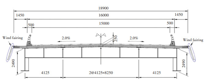
3 Example 1 — Cable-Stayed Bridge 3.1 Bridge DescriptionIn this section, a flexible cable-stayed bridge is used as an example to verify the correctness of the general expression of LRC method. The bridge has five spans with the length of 60 + 125 + 300 + 125+ 60= 670 m (Fig. 1). The bridge deck is composed of two Ⅰ-shape steel girders and a reinforced concrete slab with a total width of 18.900 m (not including the wind fairings) and a depth of 2.905 m at the center (Fig. 2). In order to improve the aerodynamic stability, a pair of wind fairings was installed on both sides of the bridge deck (Fig. 2). The two diamond-shape concrete pylons are both 91 m high. There are (2×13)×4=104 stay cables with space of 10.5 m on the deck and 1.5 m on the pylons.

|
Fig.1 General layout and support conditions of the cable-stayed bridge(Unit: m) |
|
Fig.2 Cross section of the standard bridge deck(Unit: mm) |
3.2 Dynamic Characteristics
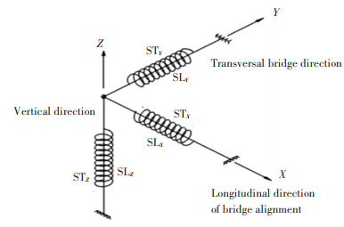
Dynamic characteristics are the fundamental properties of a structure and the basis for buffeting analysis. In this paper, finite element method is used to analyze the dynamic characteristics of the bridge. In the practice, ANSYS software was adopted to establish the finite element model of the bridge (Fig. 3). In the model, the pylons, steel girders, and piers were simulated with Beam188 element. The concrete deck slabs were simulated with Shell63 element, and the stay cables were simulated with Link10 element, in which the modulus of elasticity was modified by the Ernst formula. The pile foundations under pylons and piers were simulated by Combin14 element. Foundations of each of the pier/pylon were simulated by 6 spring elements, and the sign and corresponding equivalent stiffness of each Combin14 element are shown in Fig. 4 and Table 1 respectively, where SL and ST denote the longitudinal spring constant and the torsional spring constant. Material properties used in the finite element model are presented in Table 2.

|
Fig.3 Finite element model of the cable-stayed bridge |
|
Fig.4 General signs of stiffness for each pile foundations |
| Table 1 Equivalent stiffness of pile foundations |
| Table 2 Main parameters of material properties |
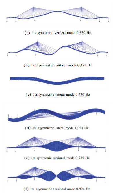
After model analysis, the dynamic characteristics are obtained. Fig. 5 shows the fundamental modes in vertical, lateral, and torsional directions of the cable-stayed bridge.
|
Fig.5 Fundamental modes in vertical, lateral, and torsional directions |
3.3 Aerodynamic Parameters
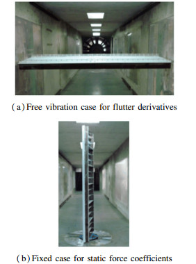
In addition to the dynamic characteristics of the bridge, aerodynamic parameters such as flutter derivatives, drag, lift, and pitching moment coefficients are also needed in buffeting analysis. Section model wind tunnel tests were carried out in TJ-1 wind tunnel of Tongji University to obtain the aerodynamic parameters. The overall arrangement of the section model test is shown in Fig. 6.
|
Fig.6 Section model tests of the cable-stayed bridge in TJ-1 wind tunnel |
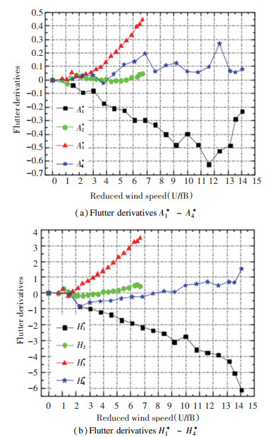
Through free-vibration case, flutter derivatives (A1*~A4*, H1*~H4*) of the bridge deck were obtained, and the values under 0 wind attack angle are shown in Fig. 7[29].
|
Fig.7 Flutter derivatives of the bridge deck under 0 wind attack angle |
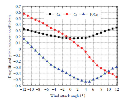
The drag, lift, and pitching moment coefficients (CD, CL, CM) were measured through force balance and the obtained values in wind-axis coordinate system are shown in Fig. 8[29]. The positive directions of wind velocity, drag force (D), lift force (L), and pitching moment (M) are illustrated in Fig. 9.
|
Fig.8 Drag, lift and pitching moment coefficients of the bridge deck (referenced to deck width B) |

|
Fig.9 Positive directions of wind velocity and wind loads acting on the bridge deck |
3.4 Buffeting Responses
After getting the structural characteristics and aerodynamic parameters of the bridge deck, the buffeting responses can be estimated using frequency domain method proposed by Davenport and Scanlan. In the calculation, the buffeting forces per unit span are expressed as[30-33]
| $ D_{\mathrm{b}}(t)=\frac{1}{2} \rho U^{2} B\left[2 C_{D} \chi_{D u} \frac{u(t)}{U}+C_{D}^{\prime} \chi_{D w} \frac{w(t)}{U}\right] $ | (16a) |
| $ L_{\mathrm{b}}(t)=\frac{1}{2} \rho U^{2} B\left[2 C_{L} \chi_{L u} \frac{u(t)}{U}+\left(C_{L}^{\prime}+C_{D}\right) \chi_{L w} \frac{w(t)}{U}\right] $ | (16b) |
| $ M_{\mathrm{b}}(t)=\frac{1}{2} \rho U^{2} B^{2}\left[2 C_{M} \chi_{M u} \frac{u(t)}{U}+C_{M} \chi_{M w}^{\prime} \frac{w(t)}{U}\right] $ | (16c) |
where the subscript b denotes buffeting; ρ is the air density; U is the mean wind velocity; C'D=dCD/dα, C'L=dCL/dα, C'M=dCM/dα; u and w are the fluctuation wind velocity components in longitudinal and vertical directions, respectively; B=18.9 m is the bridge deck width; and χDu, χDw, χLu, χLw, χMu, and χMw are the aerodynamic admittance functions, given by the simplified expression of Sears function proposed by Liepmann, as follows[34]:
| $ |\chi(K)|^{2}=\frac{1}{1+\pi K} $ | (17) |
where χ(K) is aerodynamic admittance, K=ωB/U is reduced frequency, and ω is circular frequency.
The aero-elastic forces per unit span are obtained by[32-33, 35]
| $ \begin{aligned} D_{\mathrm{ae}}=& \frac{1}{2} \rho U^{2}(2 B)\left(K P_{1}^{*} \frac{\dot{P}}{U}+K P_{2}^{*} \frac{B \dot{\alpha}}{U}+K^{2} P_{3}^{*} \alpha+\right.\\ &\left.K^{2} P_{4}^{*} \frac{p}{B}+K P_{5}^{*} \frac{\dot{h}}{U}+K^{2} P_{6}^{*} \frac{h}{B}\right) \end{aligned} $ | (18a) |
| $ \begin{aligned} L_{\mathrm{ae}}=& \frac{1}{2} \rho U^{2}(2 B)\left(K H_{1}^{*} \frac{\dot{h}}{U}+K H_{2}^{*} \frac{B \dot{\alpha}}{U}+K^{2} H_{3}^{*} \alpha+\right.\\ &\left.K^{2} H_{4}^{*} \frac{h}{B}+K H_{5}^{*} \frac{\dot{P}}{U}+K^{2} H_{6}^{*} \frac{p}{B}\right) \end{aligned} $ | (18b) |
| $ \begin{aligned} M_{\mathrm{ae}}=& \frac{1}{2} \rho U^{2}\left(2 B^{2}\right)\left(K A_{1}^{*} \frac{\dot{h}}{U}+K A_{2}^{*} \frac{B \dot{\alpha}}{U}+K^{2} A_{3}^{*} \alpha+\right.\\ &\left.K^{2} A_{4}^{*} \frac{h}{B}+K A_{5}^{*} \frac{\dot{P}}{U}+K^{2} A_{6}^{*} \frac{p}{B}\right) \end{aligned} $ | (18c) |
where the subscript ae denotes aero-elastic; the over-dot denotes the derivative with respect to time; and Pi*, Hi*, and Ai*(i=1~6) are flutter derivatives. A1*~A4* and H1*~H4* are obtained by wind tunnel tests, and the other flutter derivatives can be identified by invoking the quasi-steady theory, as follows[36]:
| $ \begin{aligned} &P_{1}^{*}=-\frac{1}{K} C_{D}, P_{2}^{*}=-\frac{1}{8 K}\left(C_{D}^{\prime}-C_{L}\right), P_{3}^{*}=\frac{1}{2 K^{2}} C_{D}^{\prime}\\ &P_{5}^{*}=\frac{1}{2 K}\left(C_{D}^{\prime}-C_{L}\right), H_{5}^{*}=\frac{1}{K} C_{L}, A_{5}^{*}=-\frac{1}{K} C_{M}\\ &P_{4}^{*}=P_{6}^{*}=H_{6}^{*}=A_{6}^{*}=0 \end{aligned} $ | (19) |
According to the Wind Resistant Design Specification for Highway Bridges[37], the air density was taken as ρ=1.225 kg/m3, the modal damping ratios were assumed as 0.01 for all modes. The height of the bridge deck above the water is z=30 m. The terrain of the bridge site can be classified into the category of type A, and the power-law index of the mean wind speed profile was 0.12. The mean wind speed at the bridge deck height with a recurrence period of 100 years can be taken as U=37.65 m/s. The roughness length z0=0.01 m. In the calculation, only the fluctuating wind load was considered.
The power spectra of u and w can be expressed as functions of n as[38]
| $ \frac{n S_{u u}(n)}{u_{*}^{2}}=\frac{200 f}{(1+50 f)^{5 / 3}} $ | (20) |
| $ \frac{n S_{w w}(n)}{u_{*}^{2}}=\frac{3.36 f}{1+10 f^{5 / 3}} $ | (21) |
where Suu(n) is the power spectrum of longitudinal velocity fluctuation, and Sww(n) is the power spectrum of vertical velocity fluctuation. n is frequency of fluctuating wind velocity, f=nz/U(z) is dimensionless frequency, z is the elevation above ground/water, u*=κU(z)/ln(z/z0) is friction velocity, and κ≈0.4 is Karman constant. An empirical formula which is suitable for engineering applications was adopted as the power cross-spectrum between u and w[39], then the power cross-spectrum Cuw(n) can be expressed as
| $ \frac{n C_{u w}(n)}{u_{*}^{2}}=\frac{14 f}{1+9.6 f^{2.4}} $ | (22) |
The span-wise correlation of the wind fluctuations can be expressed in a conventional form as[38]
| $ S\left(x_{i}, x_{j}, n\right)=S(n) \mathrm{e}^{-\frac{\lambda n}{U} \mid x_{i}-x_{j}\mid} $ | (23) |
where λ is the correlation coefficient of the wind fluctuation, according to the Chinese Wind-Resistant Code of Bridges[37], 7≤λ≤21. In the calculation, the value of λ was taken as 7. |xi-xj| is the distance between xi and xj.
In this paper, the first 20 modes are adopted to calculate the RMS values of displacement buffeting responses, and the results are shown in Fig. 10. Due to the flexibility of the bridge, background component did not dominate the buffeting responses. Both of the total and background components of the RMS values of buffeting displacements are presented in Fig. 10. Since the LRC method is just suitable to estimate background ESWL components, the background RMS values are only used to verify the general expression of the LRC method in the following sections.

|
Fig.10 RMS values of buffeting displacement of the cable-stayed bridge (Including 20 modes) |
3.5 ESWLs of the Bridge
The ESWL distributions can be obtained by LRC method through Eq.(6) or Eq.(15), and the corresponding responses can be calculated by static analysis. The correctness of the proposed general expression was verified by comparing between the calculated responses and the RMS values of the background displacement responses in Fig. 10. Seven critical nodes were set as equivalent targets, as shown in Fig. 11, in which Nodes 1, 2, 4, 6, and 7 are at the center positon of different spans, and Nodes 3 and 5 are at the quarter positon of the main span.

|
Fig.11 Equivalent nodes arrangement along the bridge (Unit: m) |
If the RMS responses for displacement at node i are taken as the equivalent target, then the ESWL distribution can be calculated. Consider that the bridge is symmetric, then only Nodes 1, 2, 3, and 4 are taken as equivalent targets.
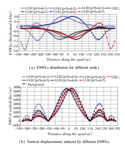
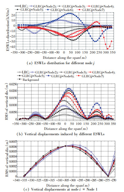
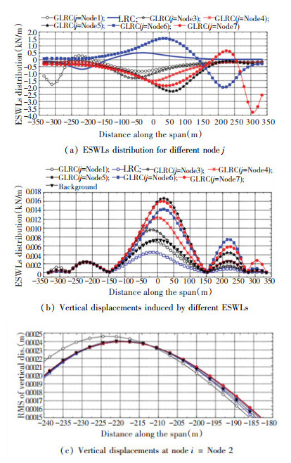
For vertical buffeting displacements, when i=Node 4 was set as the equivalent target, different ESWL distributions could be obtained through changing j by general expression of LRC method. When j=i, the general expression degenerated into the classical LRC expression. It can be found from Fig. 12(a) that the ESWL distributions were different from each other when changing j. By applying different ESWLs (Fig. 12(a)) on the bridge, the vertical displacements could be calculated by static method, as shown in Fig. 12(b). It indicates that the vertical displacement distributions were different from each other, but the values at node i=Node 4 were all equal to the background RMS vertical displacement. When i=Node 1 (Fig. 13), Node 2 (Fig. 14), and Node 3 (Fig. 15), same conclusions can be obtained.
|
Fig.12 ESWL distributions and corresponding responses for i=Node 4 in vertical direction |
|
Fig.13 ESWLs distribution and corresponding responses for i=Node 1 in vertical direction |
|
Fig.14 ESWLs distribution and corresponding responses for i= Node 2 in vertical direction |

|
Fig.15 ESWL distributions and corresponding responses for i=Node 3 in vertical direction |
For lateral buffeting displacements, when i=Node 3 was set as the equivalent target, different ESWL distributions could be obtained through changing j by general expression of LRC method. When j=i, the general expression was identical to the classical expression. From Fig. 16(a), it was found that the ESWL distributions were different from each other when changing j. If ESWLs of Fig. 16(a) is put on the bridge, then the lateral displacements could be estimated, as shown in Fig. 16(b)-(c), in which the lateral displacements for different ESWLs at node i= Node 3 were all equal to the background RMS lateral displacement. The same conclusions can be obtained for other equivalent targets of node i in lateral direction.

|
Fig.16 ESWL distributions and corresponding responses for i= Node 3 in lateral direction |
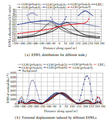
Fig. 17 presents the torsional ESWL distributions and corresponding responses for i=Node 4. In Fig. 17(a), it can be found that different node j had different ESWL distributions. Fig. 17(b) reveals that the torsional displacements at node i=Node 4 were all equal to the background RMS torsional displacement. The same conclusions can be obtained for other equivalent targets of node i in torsional direction.
|
Fig.17 ESWL distributions and corresponding responses for i=Node 4 in torsional direction |
4 Example 2 — Three Span Continuous Girder Bridge
In this section, a three span continuous girder bridge with large stiffness is used to check the correctness of the general expression of LRC method. The basic parameters of the girder bridge are shown in Table 3.
| Table 3 Main parameters of the girder bridge |
ANSYS software was used to establish the finite element model of the girder bridge, in which each span was divided into 50 elements, and only the lateral response was considered, i.e., only the degrees of the finite element model in lateral direction were investigated. Fig. 18 shows the first 6 frequencies and corresponding mode shapes of the girder bridge in lateral direction.

|
Fig.18 The first 6 frequencies and corresponding mode shapes of the girder bridge (Unit: m) |
For this example, the air density was taken as ρ=1.225 kg/m3, the mode damping ratio was assumed as 0.005 for all modes, and the drag force coefficient of the deck was taken as CD=0.1. The height of the bridge deck above the ground or water was assumed as z=30 m. The roughness length z0=0.01 m, which was taken as type A terrain conditions. The mean wind speed at the deck level was U=40 m/s. In the calculation, only the fluctuating wind in the along wind direction was considered, and the aerodynamic admittance was assumed as 1. The power spectra of u were the same as those in Eq.(20), and the span-wise correlation of u was the same as that in Eq.(23). Since the structure stiffness was large, the background component dominated the buffeting responses. In this example, the RMS responses of lateral displacement were used to represent the background buffeting responses.
For the girder bridge, 9 critical nodes were chosen as equivalent targets. Nodes 1 ~ 9 and corresponding coordinates are shown in Fig. 19.

|
Fig.19 Equivalent nodes arrangement along the girder bridge (Unit: m) |
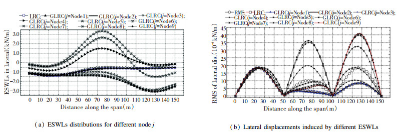
For large stiffness girder bridge, if the displacement response at the position of Node 2 was chosen as the equivalent target, different ESWLs distributions could be obtained by Eq.(20), as shown in Fig. 20(a). Fig. 20(a) reveals that for the same equivalent target of Node i, different ESWLs distributions could be acquired by changing j. When j=i, the ESWL distribution was the same as that obtained by classical expression of LRC method. Put different ESWLs to the girder bridge, then the RMS displacement responses could be obtained (Fig. 20(b)). The lateral displacements at Node 2 were all equal to the RMS values estimated by buffeting calculation method, as shown in Fig. 20(b).
|
Fig.20 ESWLs distribution and corresponding responses for i=Node 2 |
If i=Node 5 is chosen as the equivalent target, then ESWLs distributions and corresponding responses are obtained as shown in Fig. 21(a)-(b). Fig. 21 can verify the correctness of the general expression of LRC method. The same conclusions can be obtained for any other equivalent target of Node i.

|
Fig.21 ESWLs distribution and corresponding responses for i= Node 5 |
5 Example 3 — Suspension Bridge
In this section, a flexible suspension bridge with a 1000 m center span is used to check the correctness of the general expression of LRC method. In this example, 5 critical nodes were set as the equivalent targets. The general layout and the equivalent nodes arrangement of the suspension bridge are shown in Fig. 22.

|
Fig.22 Equivalent nodes arrangement along the suspension bridge (Unit: m) |
Finite element method was used in this example and the main parameters of the bridge are shown in Table 4.
| Table 4 Main parameters of the suspension bridge |
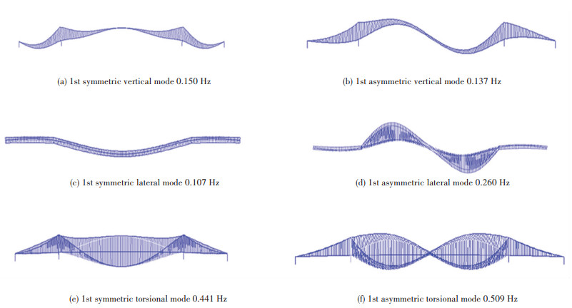
After modal analysis, the dynamic characteristics were obtained and the fundamental modes in vertical, lateral, and torsional directions are shown in Fig. 23. In the calculation, the basic parameters are shown in Table 5.
|
Fig.23 Fundamental modes in vertical, lateral, and torsional directions |
| Table 5 Basic parameters in the calculation |
The flutter derivatives (A1*~A4*, H1*~H4*) of the bridge deck under 0 wind attack angle are shown in Fig. 24[33], and the other flutter derivatives can be obtained by Eq.(19).

|
Fig.24 Flutter derivatives of the bridge deck under 0 wind attack angle |
For the flexible suspension bridge, if displacement response at the position of Node 3 (i.e., center node of the main span) was set as the equivalent target, different ESWLs distributions could be obtained by Eq.(15), as shown in Fig. 25(a), (c), and (e). From Fig. 25, it can be found that for the same equivalent target of Node 3, different ESWLs distributions could be obtained by changing j. When j=i, the ESWL distribution was the same as that obtained by the LRC method of Eq.(6). When different ESWLs acted on the suspension bridge, the RMS displacement responses could be obtained as shown in Fig. 25(b), (d), and (f), in which the vertical, lateral, and torsional displacements at the position of Node 3 were all equal to the background RMS value. If the equivalent target changes into Nodes 1, 2, 4, and 5, the same conclusions can be obtained.

|
Fig.25 ESWLs distribution and corresponding responses for i=Node 3 |
6 Conclusions
The LRC method is crucial in ESWL research and has been widely used in practice. Based on the relationship between load and response, a general expression of LRC method was derived. According to the comparison between classical and general expressions of the LRC method, three conclusions can be drawn as follows:
1) Derivation of the classical expression is based on a specific command response at a critical/concerned position, and the general expression is based on a specific command response at the entire positons. However, both expressions had the same equivalent target (
2) The classical expression is only one form of the general expression. When taking j=i in Eq.(15), the general expression was degraded into the classical expression.
3) The classical expression contains three parameters: load-response correlation coefficients, RMS values of the fluctuating wind loads, and peak factor. The general expression also introduces the response-response correlation coefficients which extend the scope of the LRC method and reveal the inherent relationship between the background ESWL distributions and the concerned parameters in an extensive way.
Finally, three different types of bridges were taken as examples to check the correctness of the general expression of LRC method. Both the theoretical derivation and the examples verified the correctness of the general expression and provided further insights into the LRC method.
In this paper, only displacement responses were used to illustrate the general expression of LRC method. In fact, other responses can also be used and similar conclusions can be obtained.
AcknowledgementThe writers are also thankful to Professor Reed at the University of Washington, Professor Zhuang Yizhou at Zhejiang Technology University, and Dr. Li Ke at Chongqing University for their comments to the manuscript.
| [1] |
Davenport A G. The application of statistical concepts to the wind loading of structures. Proceedings of the Institution of Civil Engineers, 1961, 19(4): 449-472. DOI:10.1680/iicep.1961.11304 (  0) 0) |
| [2] |
Davenport A G. The response of slender, line-like structures to a gusty wind. Proceedings of the Institution of Civil Engineers, 1962, 23(3): 389-408. DOI:10.1680/iicep.1962.10876 (  0) 0) |
| [3] |
Davenport A G. Gust loading factors. Journal of the Structural Division, 1967, 93(3): 11-34. DOI:10.1061/JSDEAG.0001692 (  0) 0) |
| [4] |
Davenport A G. The representation of the dynamic effects of turbulent wind by equivalent static wind loads. Proceedings of the 1985 International Engineering Symposium on Structural Steel. Chicago, Illinois, 1985.1-13.
(  0) 0) |
| [5] |
Irwin P A. The role of wind tunnel modeling in the prediction of wind effects on bridges. Proceedings of Bridge Aerodynamics. Balkema, Rotterdam, The Netherland, 1998.59-85.
(  0) 0) |
| [6] |
Holmes J D. Equivalent static wind load distributions for resonant dynamic response of bridges. Proceeding of the10th International Conference on Wind Engineering. Copenhagen, 1999. 907-911.
(  0) 0) |
| [7] |
Ministry of Housing and Urban-Rural Development. Load Code for the Design of Building Structures (GB 50009-2012). Beijing: China Architecture & Building Press, 2012. (in Chinese)
(  0) 0) |
| [8] |
Kasperski M, Niemann H J. The L.R.C. (load-response-correlation) - method: A general method of estimating unfavorable wind load distribution for linear and non-linear structural behavior. Journal of Wind Engineering and Industrial Aerodynamics, 1992, 43(1-3): 1753-1763. DOI:10.1016/0167-6105(92)90588-2 (  0) 0) |
| [9] |
Kasperski M. Extreme wind load distributions for linear and nonlinear design. Engineering Structures, 1992, 14(1): 27-34. DOI:10.1016/0141-0296(92)90005-B (  0) 0) |
| [10] |
Kasperski M. Extreme wind load distributions for linear and nonlinear design. Engineering Structures, 1992, 14(1): 27-34. DOI:10.1016/0141-0296(92)90005-B (  0) 0) |
| [11] |
Kasperski M. Design wind loads for low-rise buildings: A critical review of wind load specification for industrial buildings. Journal of Wind Engineering and Industrial Aerodynamics, 1996, 61(2-3): 169-179. DOI:10.1016/0167-6105(96)00051-7 (  0) 0) |
| [12] |
Holmes J D. Along-wing response of lattice towers—Ⅲ. Effective load distributions. Engineering Structures, 1996, 18(7): 489-494. DOI:10.1016/0141-0296(95)00166-2 (  0) 0) |
| [13] |
Holmes J D, Kasperski M. Effective distributions of fluctuating and dynamic wind loads. Australian Civil Engineering Transactions, 1996, 38(2-4): 83-88. (  0) 0) |
| [14] |
Zhou Y, Gu M, Xiang H F. Alongwind static equivalent wind loads and responses of tall buildings. Part Ⅰ: Unfavorable distributions of static equivalent wind loads. Journal of Wind Engineering and Industrial Aerodynamics, 1999, 79(1-2): 135-150. DOI:10.1016/S0167-6105(97)00297-3 (  0) 0) |
| [15] |
Zhou Y, Gu M, Xiang H F. Alongwind static equivalent wind loads and responses of tall buildings. Part Ⅱ: Effects of mode shapes. Journal of Wind Engineering and Industrial Aerodynamics, 1999, 79(1-2): 151-158. DOI:10.1016/S0167-6105(97)00298-5 (  0) 0) |
| [16] |
Chen X Z, Kareem A. Equivalent static wind loads for buffeting response of bridges. Journal of Structural Engineering-ASCE, 2001, 127(12): 1467-1475. DOI:10.1061/(ASCE)0733-9445(2001)127:12(1467) (  0) 0) |
| [17] |
Holmes J D. Effective static load distributions in wind engineering. Journal of Wind Engineering and Industrial Aerodynamics, 2002, 90(2): 91-109. DOI:10.1016/S0167-6105(01)00164-7 (  0) 0) |
| [18] |
Holmes J D. Wind Loading of Structures (2nd Ed). London & New York: Taylor and Francis Group, 2007.
(  0) 0) |
| [19] |
Ke S T, Ge Y J, Zhao L, et al. A new methodology for analysis of equivalent static wind loads on super-large cooling towers. Journal of Wind Engineering and Industrial Aerodynamics, 2012, 111(3): 30-39. DOI:10.1016/j.jweia.2012.08.001 (  0) 0) |
| [20] |
Ke S T, Wang T G, Ge Y J, et al. Wind-induced responses and equivalent static wind loads of tower-blade coupled large wind turbine system. Structural Engineering and Mechanics, 2014, 52(3): 485-505. DOI:10.12989/sem.2014.52.3.485 (  0) 0) |
| [21] |
Katsumura A, Tamura Y, Nakamura O. Universal wind load distribution simultaneously reproducing largest load effects in all subject members on large-span cantilevered roof. Journal of Wind Engineering and Industrial Aerodynamics, 2007, 95(9-11): 1145-1165. DOI:10.1016/j.jweia.2007.01.020 (  0) 0) |
| [22] |
Blaise N, Denoël V. Principal static wind loads. Journal of Wind Engineering and Industrial Aerodynamics, 2013, 113: 29-39. DOI:10.1016/j.jweia.2012.12.009 (  0) 0) |
| [23] |
Blaise N, Canor T, Denoël V. Reconstruction of the envelope of non-Gaussian structural responses with principal static wind loads. Journal of Wind Engineering and Industrial Aerodynamics, 2016, 149: 59-76. DOI:10.1016/j.jweia.2015.12.001 (  0) 0) |
| [24] |
Patruno L, Ricci M, de Miranda S, et al. An efficient approach to the evaluation of wind effects on structures based on recorded pressure fields. Engineering Structures, 2016, 124: 207-220. DOI:10.1016/j.engstruct.2016.06.023 (  0) 0) |
| [25] |
Patruno L, Ricci M, de Miranda S, et al. An efficient approach to the determination of equivalent static wind loads. Journal of Fluids and Structures, 2017, 68: 1-14. DOI:10.1016/j.jfluidstructs.2016.10.003 (  0) 0) |
| [26] |
Standards Australia Limited/Standards New Zealand. AS/NZS 1170.2. Structural Design Actions, Part 2: Wind actions. Sydney: SAI Global Limited. Wellington: Standards New Zealand, 2002.
(  0) 0) |
| [27] |
ISO (The International Organization for Standardization). ISO 4354: 2009. Wind Actions on Structures. Geneva: ISO. 2009.
(  0) 0) |
| [28] |
Dong R, Ge Y J, Yang Y X, et al. Multi-target equivalent static wind loads of long-span bridges based on proper orthogonal modes. China Civil Engineering Journal, 2019, 52(7): 110-117. (in Chinese) DOI:10.15951/j.tmgcxb.2019.07.011(inChinese) (  0) 0) |
| [29] |
Yang Yongxin, Dong Rui. Wind Tunnel Study on Wind-Resistant Performance of Co Chien Cable-Stayed Bridge in Vietnam (Research Report). Shanghai: Tongji University, 2011.
(  0) 0) |
| [30] |
Davenport A G. Buffeting of a suspension bridge by storm winds. Journal of Structure Engineering-ASCE, 1962, 88(3): 233-270. (  0) 0) |
| [31] |
Scanlan R H. The action of flexible bridges under wind, Ⅱ: Buffeting theory. Journal of Sound and Vibration, 1978, 60(2): 201-211. DOI:10.1016/S0022-460X(78)80029-7 (  0) 0) |
| [32] |
Scanlan R H. Problematics in formulation of wind-force models for bridge decks. Journal of Engineering Mechanics-ASCE, 1993, 119(7): 1353-1375. DOI:10.1061/(ASCE)0733-9399(1993)119:7(1353) (  0) 0) |
| [33] |
Ding Q S. Refinement of Coupled Flutter and Buffeting Analysis for Long-span Bridges. Shanghai: Tongji University, 2001. (in Chinese)
(  0) 0) |
| [34] |
Liepmann H W. On the application of statistical concepts to the buffeting problem. Journal of the Aeronautical Sciences (Institute of the Aeronautical Sciences), 1952, 19(12): 793-800. DOI:10.2514/8.2491 (  0) 0) |
| [35] |
Scanlan R H. The action of flexible bridges under wind, I: Flutter theory. Journal of Sound and Vibration, 1978, 60(2): 187-199. DOI:10.1016/S0022-460X(78)80028-5 (  0) 0) |
| [36] |
Chen X Z, Matsumoto M, Kareem A. Aerodynamic coupling effects on flutter and buffeting of bridges. Journal of Engineering Mechanics-ASCE, 2000, 126(1): 17-26. DOI:10.1061/(asce)0733-9399(2000)126:1(17) (  0) 0) |
| [37] |
Ministry of Communications and Transportation. JTG/T D60-01-2004. Wind-resistant Design Specification for Highway Bridges. Beijing: Ministry of Communications and Transportation, 2004. (in Chinese)
(  0) 0) |
| [38] |
Simiu E, Scanlan R H. Wind Effects on Structures: Fundamentals and Applications to Design (3rd Ed). New York: John Wiley & Sons, Inc., 1996.
(  0) 0) |
| [39] |
Kaimal J C, Wyngaard J C, Izumi Y, et al. Spectral characteristics of surface-layer turbulence. Quarterly Journal of the Royal Meteorological Society, 1972, 98(417): 563-589. DOI:10.1002/qj.49709841707 (  0) 0) |
 2021, Vol. 28


