2. College of Mechanical Engineering, Yanshan University, Qinhuangdao 066004, Hebei, China;
3. School of Electrical Engineering, Yanshan University, Qinhuangdao 066004, Hebei, China;
4. Beijing Institute of Space Mechanic & Electricity, Beijing 100094, China
Hyperspectral images contain a large amount of spectral information and it can collect radiation information in the ultraviolet, visible, near-infrared, and mid-infrared regions of the electromagnetic spectrum, achieving perfect combination of space and spectrum[1]. Hyperspectral image classification (HSIC) techniques are commonly used in agriculture[2], chemical imaging, and environment science[3]. However, the hyperspectral image has high-dimensional spectrum and redundant information which can cause Hughes phenomenon generally[4].
HSIC has attracted considerable attentions in the field of remote sensing image processing. In traditional HSIC methods, support vector machine (SVM) is commonly applied[5], which only considers the image spectral information. Kang et al.[6] proposed the sobel edge detection algorithm, which uses spatial information to consider the information discontinuity in the multi-dimensional dataset. As a preprocessing method, it can reduce noise and improve class separability in the spectral dimensionality. As a post-processing step, it can work on the labelled image or classification probability obtained from the pixel-level classifier. Li et al.[7] proposed an HSIC framework based on ERW. It firstly used SVM to obtain the classification probability map, then used the ERW algorithm to optimize the obtained pixel category probability map. Li et al.[8] introduced convolutional sparse representation to improve the classification performance. But these HSIC methods usually require complex feature extraction processes.
Because of the excellent expressiveness of deep learning models in various image processing tasks, they are gradually applied to HSIC. Chen et al.[3] made use of stacked autoencoders to extract the discriminative features of hyperspectral images, then used logistic regression for classification. Although SAE can extract depth features by layers, the training pixels need to be expanded to one dimension to satisfy the input requirements of the fully connected layer. As a result, image information may be lost.
Convolutional neural networks (CNN) can actively learn rich features from original data, guarantee the integrity of spatial and spectral information, and avoid the randomness of artificial feature extraction[9].For the purpose of effectively extracting representative features from complex scenes, a dual path network (DPN) is proposed, which combines residual network and fully convolutional network[10]. Niu et al.[11] utilized DeepLab to extract the spatial features at multiple scales and fused them with spectral features for HSIC.
2D-CNN-based methods usually need to extract spatial and spectral information separately, requiring preprocessing such as principal component analysis (PCA) for image spectral dimensions. Zhong et al.[12] constructed a spatial spectrum residual network (SSRN) based on 3D-CNN, and designed continuous spatial and spectral residual modules, achieving high classification performance. However, 3D-CNN is able to sample in both spatial and spectral dimensions, so designing feature extraction modules separately makes the network design redundant. In order to decrease training time and increase accuracy, an HSIC framework based on fast dense spectral-spatial convolution (FDSSC) was proposed, using "valid" convolution to decrease dimensionality[13]. Based on the idea of maximizing the utilization rate of image information, Zhao and Yang[14] proposed an improved 3D convolutional neural network classification framework, which was suitable for the 3D data of hyperspectral images. Because of the high-dimensional spectrum of hyperspectral images and the limited number of labeled samples, the above methods still face the problem of information loss.
Based on previous research, multi-scale dilated convolutional neural network (MDCNN) is proposed, which can effectively avoid information loss and increase the HSIC accuracy. The major contributions are summarized as follows:
1) In the image segmentation method, dilated convolution is used in convolutional neural network to classify hyperspectral images, extracting more extensive and abstract image features. Dilated convolution can prevent the reduction of image resolution, expand the receptive field of filters, and obtain multi-scale features.
2) A multi-scale dilated convolutional neural network (MDCNN) is proposed to extract spatial- spectral features, which can obtain excellent classification results. Multi-scale aggregate structure is constructed, which uses shortcut connection and dilated convolution in each channel, effectively extracts image features, avoids information loss, and prevents over-fitting.
3) The effectiveness of MDCNN is verified by conducting comprehensive comparison on two public hyperspectral datasets. The results show that MDCNN is superior to four existing methods.
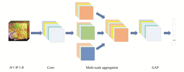
1 MDCNN FrameworkGenerally, in CNN, convolutional layers and pooling layers are stacked on top of each other. During the network training, too many subsampling operations can result in the loss of sample information. For this problem, dilated convolution is applied to HSIC, and a classification framework based multi-scale dilated convolutional neural network (MDCNN) is proposed. The MDCNN structure is shown in Fig. 1.
|
Fig.1 Architecture of the MDCNN |
1.1 First-Layer Spectral Dimension Reduction
MDCNN mainly consisted of three parts: first-layer spectral dimension reduction, multi-scale aggregation, and a global average pooling (GAP) layer. Firstly, the convolutional step size of the spectral dimension was used to extract shallow spatial-spectral information while reducing the image dimensionality. Then, there was a multi-scale aggregation structure. Multi-scale discriminant image features were extracted by using different dilated rates, and over-fitting was prevented by adding shortcut connection to each channel. Finally, the global average pooling layer was used for network optimization. The final features were input into Softmax for classification.
MDCNN selected the first convolutional layer to reduce spectral dimension by using step size. It used 1×1×n filter, where the spatial convolution step was 1×1, and the convolution step of the spectral dimension was set to c. As a result, the stage of data preprocessing was omitted and the loss of image information was avoided.
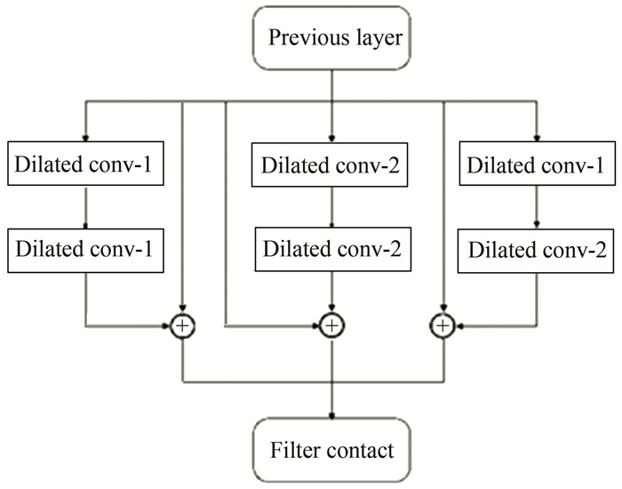
1.2 Multi-Scale AggregationFor the purpose of reducing the loss of information during image feature extraction, a special structure, multi-scale aggregate, is proposed, which is similar to the Inception module[15]. It contained three channels, and each channel contained two convolutional layers. The shortcut connection in the residual network was used in each channel. The purpose of this design is to decrease the probability of weak signal loss, extract the depth image features, and avoid the over-fitting phenomenon. The step of using shortcut connection can accelerate convergence and improve generalization ability. The multi-scale aggregation structure can effectively extract the context multi-scale discriminant features and better perform the target classification task.
In the process of semantic segmentation, repeating pooling operations may decrease image resolution or cause information loss. Dilated convolution provides a new approach to expand the receptive field while ensuring that the resolution does not decrease. Also, it comes up with an improved means of acquiring multi-scale contextual features through distinct dilated rates. Inspired by this, each channel of the multi-scale aggregation structure used different dilated rates: the first channel used standard convolutional layers, i.e., r=1. The second channel convolutional layers' dilated rate was r=2, and the third channel adopted standard convolution and dilated convolution stacking structure. The structure of multi-scale aggregation is shown in Fig. 2. Dilated conv-i represents a dilated convolutional layer whose dilated rate equals i.
|
Fig.2 Schematic of the multi-scale aggregation |
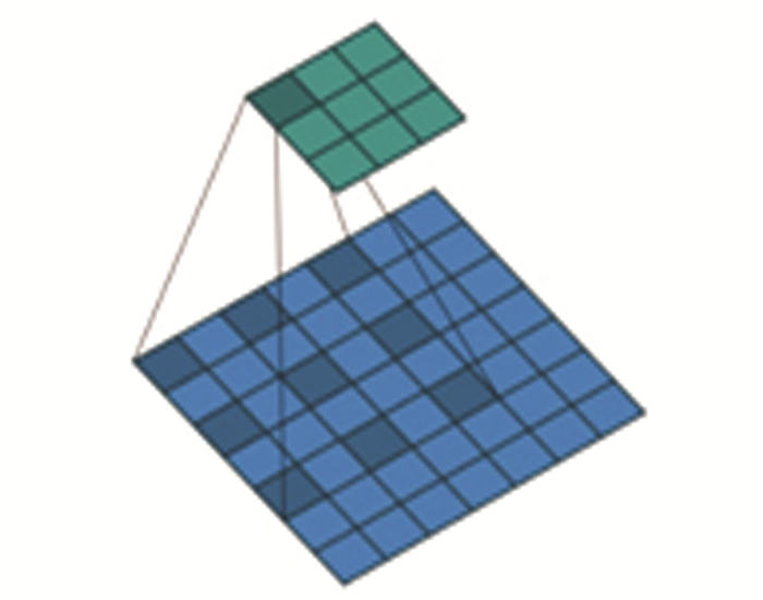
Standard convolution is to perform convolution operation on adjacent elements of the image local features, which is a continuous operation. Dilated convolution injects dilation into the filter, so that there is a gap between the convolution elements. The convolution operation was performed in a jumping manner, which expands the range of the receiving domain.
Fig. 3 illustrates an example of 2D dilated convolution. The convolution kernel size was 3×3. The dilated rate was set to 2. As a result, the receptive field of each element in the feature map was 7×7. Generally speaking, the receptive field size was computed as follows:
| $ \begin{array}{l} {F_r} = \left( {{2^{i + 2}} - 1} \right) \times \left( {{2^{i + 2}} - 1} \right){\rm{, }}\\ \;i = {\rm{max}}\{ j|{2^j} \le r, j \in M\} \end{array} $ | (1) |
|
Fig.3 Illustration of the dilated convolution |
where Fr is the receptive field size, r is the rate corresponding to the stride with which the input signal can be sampled, and M represents the set of natural numbers.
1.3 Global Average Pooling LayerIn view of convolutional neural networks, fully connected layers are generally used at the end of network in HSIC. Its main function is to stretch the extracted features by the last layer into a 1-D vector. Then it is input to Softmax to be classified. In this process, there are too many parameters in the fully connected layer, which reduces the training speed and is prone to over-fitting. In order to prevent over-fitting, the global average pooling layer was used at the end of the network to regularize the entire network. The operation of directly deleting the black box in the fully connected layer can achieve image input of any size.
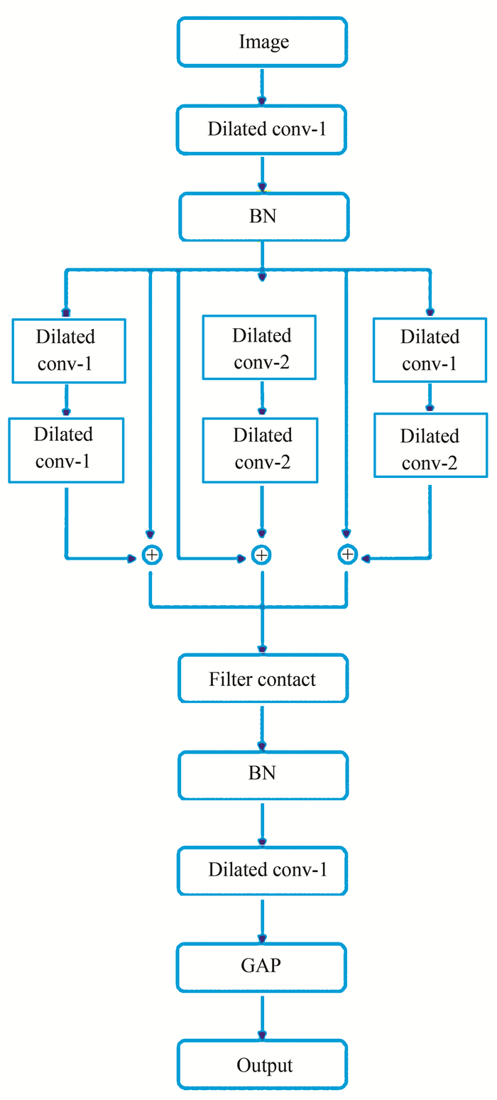
1.4 Parameters SetMDCNN used s×s×B 3D data blocks as input samples, where s×s represents the spatial size of pixel block obtained by slicing, and B is the spectral dimension of dataset. The detail is revealed in Fig. 4.
|
Fig.4 Schematic diagram of MDCNN |
There were 8 convolutional layers and 1 global average pooling layer totally. Except that the first layer used 1×1×11 filter, all other layers used 3×3×3 filter. The number of filters was set to 32 in all convolutional layers. At the end, the feature map was transformed into 1×C vector by global average pooling layer. The index of the largest value in the vector represents the predicted label of the input image through the Softmax layer. BatchNormalization (BN) was added in the last of each part to prevent over-fitting. In addition, the rectified linear unit (ReLU) has a huge acceleration effect on the convergence of stochastic gradient descent. So the non-linear activation function of ReLU was utilized:
| $ f\left( x \right) = {\rm{max}}(0, x) $ | (2) |
In order to learn the proposed network MDCNN, the categorical cross entropy was selected as the loss function. The stochastic gradient descent (SGD) was chosen to optimize network parameters. The learning rate, weight decay, and momentum were set to 0.01, 0.0005, and 0.9, respectively. The training batch size was set to 16 in 1000 iterations.
2 DatasetsThe proposed network, MDCNN, was trained on two popular hyperspectral datasets: the Indian Pines dataset and the Pavia University dataset.
The Indian Pines dataset is imaged by AVIRIS on an Indian pine tree, which contains 145×145 pixels and 200 valid spectral bands for classification and the spatial resolution is 20 m. There are 10249 labeled pixels totally, which consists of 16 classes.
The Pavia University dataset is a part of hyperspectral data obtained by the ROSIS sensor from main urban area of Pavia in 2003. The data size is 610×340×103, when the noisy bands have been discarded. It contains 42776 labeled sample pixels with 9 ground truth classes, including roads, trees, and roofs.
3 Experiments and ResultsFor the purpose of evaluating proposed network performance, four other HSIC methods, including SVM[16], SAE[3], 2DCNN[17], and 3DCNN[18] were compared. The classification indexes used the overall accuracy (OA), average accuracy (AA), and Kappa statistics.
OA indicates the proportion of the number correctly classified to the total number of the input data. The higher the ratio, the higher the classification ability of the network. The calculation formula is shown in Eq. (3):
| $ {\rm{OA}} = \frac{{\sum\limits_{i = 1}^c {{N_{ii}}} }}{N} $ | (3) |
where Nii indicates the number that the input samples belong to the i category and the predicted result is still the i category. N indicates the total number of pixels.
AA refers to the average value of the classification accuracy of each feature category, which measures the classification ability of the model from the category level, as shown in Eq. (4):
| $ {\rm{AA}} = \frac{{\sum\limits_{i = 1}^c {\frac{{{N_{ii}}}}{{{N_{i\;*}}}}} }}{C} $ | (4) |
where Ni* indicates the number of samples belonging to category i, C is the total number of pixel categories in the hyperspectral dataset.
Kappa coefficient is an index to determine classification accuracy. It can measure the degree of agreement between the predicted classification result and the real label. The value range is [-1, 1], and the actual output range is [0, 1]. The formula is shown in Eq. (5):
| $ {\rm{Kappa}} = \frac{{N\sum\limits_{i = 1}^c {{N_{ii}} - \sum\limits_{i = 1}^c {{N_{i*}}{N_{*i}}} } }}{{{N^2} - \sum\limits_{i = 1}^c {{N_{i*}}{N_{*i}}} }} $ | (5) |
where Nij is the element value of the i row and j column in the confusion matrix. Ni* and N*i represent the total number of samples in the i row and j column, respectively.
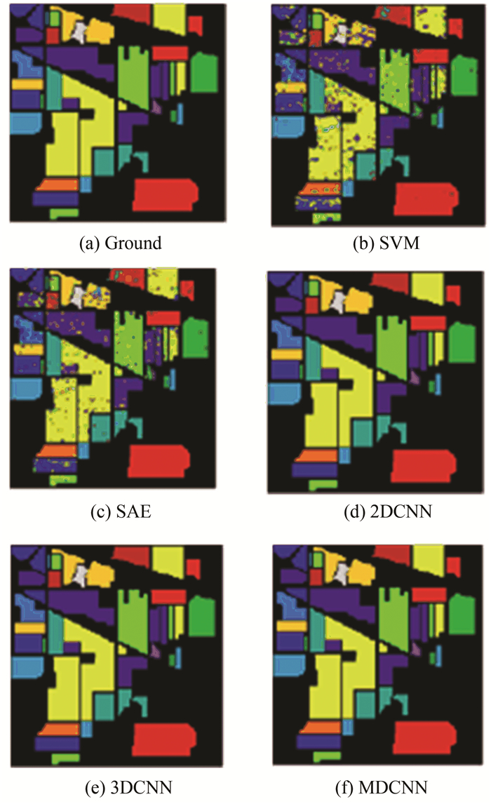
3.1 Indian Pines Experimental ResultsThe first experiment was conducted on the Indian Pines dataset. For all methods, 20% labeled samples were selected randomly as training data to train the network. The input size was 9×9×200. The comparison of the experimental classification results with several considered comparison methods are presented in Table 1, which shows MDCNN achieved remarkable improved accuracy. Compared with the SVM method, CNN can learn deep-level features autonomously, which had 17.45% improvement of OA and 17.6% of AA. For the unsupervised method named SAE, MDCNN can use the label information to obtain discriminative classification features, improving classification accuracy by 13.49%. 2DCNN adopted the original stacked convolution, while MDCNN used dilated convolution in multi-scale aggregation to increase OA by 2.1%. Compared with the 3DCNN using the double convolution pooling structure, MDCNN extracted deeper spatial-spectral features, achieving the highest OA value of 99.58% and the AA value of 99.57%. Experimental data clearly show that MDCNN is more competitive in HSIC tasks.
| Table 1 Comparative classification results with different methods for the Indian Pines scene |
Among the 16 individual categories in total, the classification accuracy of 15 categories achieved the highest accuracy. Especially in the 4th category stone-steel-towers, the 9th category Oats, the 14th category woods, and the 15th category bldg-grass-tree-drives, they reached 100% classification accuracy, achieving completely correct classification.
The classification map of all methods is illustrated in Fig. 5. It can be noticed that the classification map of SVM and SAE was greatly affected by noise and the classification performance was poor. For 2DCNN and 3DCNN, there were still many misclassifications. MDCNN significantly reduced the impact of noise, achieved high classification performance, and had a stable classification effect.
|
Fig.5 Classification maps of the Indian Pines dataset |
3.2 Pavia University Experimental Results
For the Pavia University dataset, the ratio of training set to the test set was 1∶9, and the input size was set to 7×7×103. The mean classification results of several comparison methods are given in Table 2. At the same time, the corresponding classification maps are shown in Fig. 6. It can be seen that the MDCNN framework is superior to other methods. Specifically, the OA value of MDCNN reached 99.92%, which was 9.38%, 5.19%, 0.78%, and 1.05% higher than SVM, SAE, 2DCNN, and 3DCNN, respectively. The AA value also reached 99.90%, achieving high classification performance.
| Table 2 Comparative classification results with different methods for the Pavia University scene |

|
Fig.6 Classification maps of the Pavia University dataset |
In the nine categories of the dataset, the classification accuracy of each category was as high as 99% or more. Even the classification results of five categories such as meadows, painted metal sheets, bare soil, bitumen, and shadows achieved high accuracy value of 100%. The experimental results fully show the superiority of the classification performance of MDCNN.
Fig. 6 shows the classification maps of SVM and SAE with serious misclassification. Although the classification accuracy of the 2DCNN and 3DCNN methods was improved, the classification map of MDCNN was closer to the real ground.
4 ConclusionsIn order to solve the problem of image classification reduction caused by the loss of image resolution and improve the performance of HSIC, a framework based dilated convolutional neural network is proposed and a novel structure is proposed which combines shortcut connection with multi-scale. Dilated convolution was introduced to HSIC without losing resolution for improving classification accuracy. To overcome the degradation problem in learning process, BN layer was utilized for a good generalization. The obtained experimental results demonstrate that MDCNN provides quantitative improvements, indicating that it extracts more distinctive features to conduct effective classification.
There are still some problems in HSIC to be discussed and solved. In our next study, the HSIC task can be considered in unsupervised settings.
| [1] |
Bioucas-Dias J M, Plaza A, Camps-Valls G, et al. Hyperspectral remote sensing data analysis and future challenges. IEEE Geoscience and Remote Sensing Magazine, 2013, 1(2): 6-36. DOI:10.1109/MGRS.2013.2244672 (  0) 0) |
| [2] |
Wang D, Wu J. Study on crop variety identification by hyperspectral remote sensing. Geography and Geo-information Science, 2015, 31(2): 29-33. DOI:10.3969/j.issn.1672-0504.2015.02.007 (  0) 0) |
| [3] |
Chen Y S, Lin Z H, Zhao X. Deep learning-based classification of hyperspectral data. IEEE Journal of Selected Topics in Applied Earth Observations and Remote Sensing, 2014, 7(6): 2094-2107. DOI:10.1109/JSTARS.2014.2329330 (  0) 0) |
| [4] |
Wang L Z, Zhang J B, Liu P, et al. Spectral-spatial multi-feature-based deep learning for hyperspectral remote sensing image classification. Soft Computing, 2017, 21(1): 213-221. DOI:10.1007/s00500-016-2246-3 (  0) 0) |
| [5] |
Peng J T, Zhou Y C, Chen C L P. Region-kernel-based support vector machines for hyperspectral image classification. IEEE Transactions on Geoscience and Remote Sensing, 2015, 53(9): 4810-4824. DOI:10.1109/TGRS.2015.2410991 (  0) 0) |
| [6] |
Kang X D, Li S T, Fang L Y, et al. Extended random walker-based classification of hyperspectral images. IEEE Transactions on Geoscience and Remote Sensing, 2015, 53(1): 144-153. DOI:10.1109/TGRS.2014.2319373 (  0) 0) |
| [7] |
Li J, Khodadadzadeh M, Plaza A, et al. A discontinuity preserving relaxation scheme for spectral-spatial hyperspectral image classification. IEEE Journal of Selected Topics in Applied Earth Observations and Remote Sensing, 2016, 9(2): 625-639. DOI:10.1109/JSTARS.2015.2470129 (  0) 0) |
| [8] |
Li H C, Zhou H L, Pan L, et al. Gabor feature-based composite kernel method for hyperspectral image classification. Electronics Letters, 2018, 54(10): 628-630. DOI:10.1049/el.2018.0272 (  0) 0) |
| [9] |
Ouyang N, Zhu T, Lin L P. Convolutional neural network trained by joint loss for hyperspectral image classification. IEEE Geoscience and Remote Sensing Letters, 2019, 16(3): 1-5. DOI:10.1109/LGRS.2018.2872359 (  0) 0) |
| [10] |
Kang X D, Zhuo B B, Duan P H. Dual-path network-based hyperspectral image classification. IEEE Geoscience and Remote Sensing Letters, 2019, 16(3): 1-5. DOI:10.1109/LGRS.2018.2873476 (  0) 0) |
| [11] |
Niu Z J, Liu W, Zhao J Y, et al. DeepLab-based spatial feature extraction for hyperspectral image classification. IEEE Geoscience and Remote Sensing Letters, 2019, 16(2): 251-255. DOI:10.1109/LGRS.2018.2871507 (  0) 0) |
| [12] |
Zhong Z L, Li J, Luo Z M, et al. Spectral-spatial residual network for hyperspectral image classification: a 3-D deep learning framework. IEEE Transactions on Geoscience and Remote Sensing, 2018, 56(2): 847-858. DOI:10.1109/TGRS.2017.2755542 (  0) 0) |
| [13] |
Wang W J, Dou S G, Jiang Z M, et al. A fast dense spectral-spatial convolution network framework for hyperspectral images classification. Remote Sensing, 2018, 10(7): 1068-1087. DOI:10.3390/rs10071068 (  0) 0) |
| [14] |
Zhao Y, Yang Q J. Research on hyperspectral remote sensing image classification based on 3D convolutional neural network. Information Technology and Network Security, 2019, 38(6): 46-51. (  0) 0) |
| [15] |
Szegedy C, Liu W, Jia Y Q, et al. Going deeper with convolutions. 2015 IEEE Conference on Computer Vision and Pattern Recognition (CVPR). Piscataway: IEEE, 2015, 1-9. DOI:10.1109/CVPR.2015.7298594 (  0) 0) |
| [16] |
Waske B, van der Linden S, Benediktsson J A, et al. Sensitivity of support vector machines to random feature selection in classification of hyperspectral data. IEEE Transactions on Geo-Science and Remote Sensing, 2010, 48(7): 2880-2889. DOI:10.1109/TGRS.2010.2041784 (  0) 0) |
| [17] |
Hu W, Huang Y Y, Wei L, et al. Deep convolutional neural networks for hyperspectral image classification. Journal of Sensors, 2015, 2015: 258619. DOI:10.1155/2015/258619 (  0) 0) |
| [18] |
Li G D, Zhang C J, Gao F, et al. Doubleconvpool-structured 3D-CNN for hyperspectral remote sensing image classification. Journal of Image and Graphics, 2019, 24(4): 639-654. DOI:10.11834/jig.180422 (  0) 0) |
 2021, Vol. 28


