2. Key Laboratory of Enhanced Oil Recovery (Northeast Petroleum University), Ministry of Education, Daqing 163318, Heilongjiang, China;
3. The Fourth Oil Production Factory, Daqing Oilfield Corporation Ltd., Petro China, Daqing 163511, Heilongjiang, China
The focus of non-Newtonian flows research is the quantification of turbulence in mechanical and engineering fields, such as coal water slurry transport, drilling fluid carrying cuttings, polymer transportation and processing of its products, pulp suspension flow and blood flow in thoracic aorta[1-3]. The studies on non-Newtonian fluids turbulence are critical to the pipeline transportation of oil and gas to reduce drag and save energy. Such turbulence is capable of restricting the energy consumption and simplifying pump station settings[4-5]. As compared with Newtonian fluid, the turbulence theory and numerical approaches of non-Newtonian fluids are still underdeveloped[6]. Some attempts have been made regarding the effects of the rheological parameter and Reynolds number on the flow behavior. The numerical models of non-Newtonian fluids make up for the deficiencies of the existing theory, and develop the turbulence theory of non-Newtonian fluids.
The research on the non-Newtonian flow behavior make some progress with experiments. By studying different concentrations of polymer solutions, Pinho and Whitelaw[7] demonstrated that shear thinning could cause delays in the transition from laminar to turbulent flow and inhibit turbulent fluctuations. Bogue and Metzner[8] conducted a comprehensive review on the prior art data of the Newton velocity profile, and then they empirically corrected the conventional correlation based on ascertained velocity profiles of the turbulent core regions for Newtonian fluid and non-Newtonian fluids. Rudman et al.[9] found that analogous phenomena to jets and slugs in Newtonian fluid occurred in transition turbulence of non-Newtonian fluids.
With the development of computer and the increase of calculation, it is entirely feasible to obtain some detailed information of turbulence by numerical simulation for non-Newtonian fluids flow, but it is difficult to obtain some flow information by experiments. The methods of numerical simulation consist of direct numerical simulation (DNS), large eddy simulation (LES), and Reynolds averaged Navier-Stokes (RANS). DNS maintains advantages in high precision, but it needs high spatial, temporal resolution and cost. Besides, RANS is simple in its computation, but it faces difficulty in acquiring specific turbulence information. In comparison, LES is a more suitable method, which is capable of regenerating the main turbulence structures by separating large-scale vortices from small-scale vortices with a filtering function under reasonable computational expense[10-11]. The basic idea is to calculate the large-scale pulsation directly, but only the small-scale pulsation is modeled. Therefore, for the first step of LES, the small-scale pulsation is to be filtered out by a filtering function, by which the unsteady structures are captured without high computational expense compared with direct numerical simulation[12]. Dairay et al.[13] adopted a coarser to perform LES on the pipeline turbulence. Their results revealed that the mean velocity and Reynolds stress near the wall comply with the direct numerical simulation without considering near-wall model. Cheng and Samtaney[14] characterized the mean velocity distribution, velocity gradient, and scaled velocity gradient ratio on the zero-pressure gradient boundary layer, suggesting that the mean velocity of near-wall turbulence was closer to logarithmic law based on the quantitative analysis. With the approximate temporal deconvolution method, Thais et al.[15] proposed temporal LES on turbulence of viscoelastic fluid, by which the high anisotropy of turbulence was regenerated, and the results had a good consistency with direct numerical simulation in terms of drag reduction prediction. The subgrid-scale model is the most important part to LES. The accuracy of numerical simulation, especially for anisotropic turbulence, is primarily determined by the selection of subgrid-scale model. In general, the subgrid-scale models include the Smagorinsky model, the dynamic Smagorinsky-Lilly model, the Scale-similar subgrid model, and so on. At present, in order to increase the applicability for various models, many researchers are still working on the development of subgrid-scale model. Molla and Paul[16] assessed several viscosity models for the non-Newtonian blood flow in accordance with the results of the dynamic subgrid-scale model constant, as well as relative subgrid-scale normalized viscosity. According to the DNS results, Ohta and Miyashita[12] proposed an extended Smagorinsky model to correct the filter width of local viscosity changes, which could precisely predict the subgrid-scale stress of shear thickening and shear thinning. Gnambode et al.[17] respectively illustrated the effects of single variation (power-law index and Reynolds numbers) on the turbulence of power-law fluids in a circular pipe, and confirmed the feasibility of LES in assessing the turbulence of power-law fluids with a higher Reynolds number.
The flow behaviors of non-Newtonian fluids in pipes have been extensively applied in practical industries. The purpose of this study is to explore the effects of power-law index on fluid turbulence in pipes based on subgrid-scale model. The distributions of mean velocity, friction coefficient, normalized viscosity, root mean squares (RMS) of the fluctuation velocity, Reynolds stress, and higher-order statistics were obtained. Furthermore, the validity of LES method in predicting turbulent flow for power-law fluids pipelines was tested by comparing simulation results by Gnambode et al.[17] and Khoury et al.[18]
1 Numerical Method 1.1 Governing EquationsThe object of study is the turbulence of power-law fluids in a circular pipe. The spatial discretisation is based on the element-Fourier of spectral formulation, and the boundary conditions utilize axial periodic boundary conditions. The dimensionless filtering incompressible continuity and momentum equations are expressed as
| $ \frac{{\partial {{\bar u}_i}}}{{\partial {x_i}}} = 0 $ | (1) |
| $ \begin{array}{l} \frac{{\partial {{\bar u}_i}}}{{\partial t}} + \frac{{\partial {{\bar u}_i}{{\bar u}_j}}}{{\partial {x_j}}} = - \frac{{\partial \bar p}}{{\partial {x_i}}} + \\ \ \ \ \ \ \ \ \ \ \frac{1}{{{\rm{R}}{{\rm{e}}_s}}}\frac{\partial }{{\partial {x_j}}}\left[ {\dot \gamma _d^{n - 1}(\frac{{\partial {{\bar u}_i}}}{{\partial {x_j}}} + \frac{{\partial {{\bar u}_j}}}{{\partial {x_i}}})} \right] - \frac{{\partial {{\bar \tau }_{ij}}}}{{\partial {x_j}}} \end{array} $ | (2) |
where xi, xj denote the spatial coordinates;
Dynamic Smagorinsky-Lilly model was employed as a dynamic method to determine the reference model coefficients, which was proposed by Germano et al.[19] and improved by Lilly[20]. The basic idea is to introduce local turbulent structures information into subgrid stress using twice filtering, and then adjust model coefficients in the calculation process. The dynamic model coefficient is determined based on the local characteristics of the solvable scale fluctuations. Compared with the Smagorinsky-Lilly model, the dynamic model addresses the excessive dissipation caused by single constant in Smagorinsky-Lilly model.
The subgrid stress tensor τij is defined as
| $ {\bar \tau _{ij}} = - 2v{\bar S_{ij}} = - 2{C_d}{\mathit{\Delta }^2}{\left[ {2{{\bar S}_{ij}}{{\bar S}_{ij}}} \right]^{1/2}}{\bar S_{ij}} $ | (3) |
where vt denotes subgrid-scale turbulent viscosity; △ is the computational filter; the strain rate tensor is
| $ {\bar S_{ij}} = \frac{1}{2}\left[ {\frac{{\partial {{\bar u}_i}}}{{\partial {{\bar u}_j}}} + \frac{{\partial {{\bar u}_j}}}{{\partial {{\bar u}_i}}}} \right] $ | (4) |
Cd is the dynamic coefficient replacing Smagorinsky coefficient. The dynamic model coefficient Cd is expressed as
| $ {C_d} = {\rm{ - }}\frac{1}{{2{\mathit{\Delta }^2}}}\frac{{\left\langle {{L_{ij}}{M_{ij}}} \right\rangle }}{{\left\langle {{M_{ij}}{M_{ij}}} \right\rangle }} $ | (5) |
Here, the superscript 〈(·)〉 denotes statistically averaged value, and the tensors Lij and Mij are defined as
| $ {L_{ij}} = \widetilde {{{\bar q}_i}{{\bar q}_j}}{\rm{ - }}\widetilde {{{\bar q}_i}}\widetilde {{{\bar q}_j}} = - 2{C_d}{\mathit{\Delta }^2}{M_{ij}} $ | (6) |
| $ {M_{ij}} = \frac{{\widetilde {{\mathit{\Delta }^2}}}}{{{\mathit{\Delta }^2}}}\widetilde {|\bar S|{{\bar S}_{ij}}}{\rm{ - }}\widetilde {|\bar S|{{\bar S}_{ij}}} $ | (7) |
where the size of the test filter with the superscript should be larger than the grid filter △=(r△r△θ△z)1/3.
1.3 Boundary ConditionsThe computational domain is the horizontal smooth circular pipe with its length of 10R, as shown in Fig. 1. The axial and circumferential grids are uniform, while the radial grids are non-uniform. In wall-bounded turbulence, viscous sublayer, and buffer layer play an important role in turbulent energy regeneration. To obtain accurate solution, the grid resolution should be finer near the wall (y+ < 1). For present LES, by simulating the different power-law indexes at ReMR=20000, the near-wall mesh spacing is found as y+ < 0.1 in all cases, complying with the grid resolution of previous requirement, as shown in Table 1. On the viscous sublayer, there are approximately 10 gridpoints. Thus, the accuracy of the mesh in this simulation is sufficient to obtain the momentum transport at the wall. In DNS calculation, the number of grids should reach Re9/4[11]. The number of grids in DNS (437×106) is about 383 times that of the LES (1.14×10⁶) at the Reynolds number of 20000[18]. In comparison, the computational cost of LES decreases considerably. It is assumed that the turbulence statistics of the circular pipe are periodic following the circumferential and axial directions. Moreover, the inlet and outlet of a circular pipe are assumed as displacement periodic boundary conditions, and the wall surface adopts the non-slip boundary conditions to fully develop the turbulence.

|
Fig.1 Computational domain for fully developed turbulence in a horizontal pipeline |
| Table 1 Parameters and grid scale of present LES simulations |
The calculation of the Reynolds number of non-Newtonian fluids follows Newtonian fluid. However, as the viscosity varies with time and space, the Reynolds number calculated is inaccurate based on the appropriate viscosity scale[6]. In this study, Metzner-Reed Reynolds number was adopted to calculate generalized Reynolds number of power-law fluids:
| $ {\rm{R}}{{\rm{e}}_{{\rm{MR}}}} = \frac{{\rho {D^n}u_b^{2{\rm{ - }}n}}}{{\frac{K}{8}{{\left( {\frac{{6n + 2}}{n}} \right)}^n}}} $ | (8) |
where ub is the bulk velocity; D is pipe diameter.
y+=ρuτ(r-R)/ηw is the non-dimensional distance from the wall, where R = D/2 is the pipe radial. u+=u/uτ is defined as the non-dimensional velocity. The friction velocity is uτ=(τw/ρ)1/2, and the mean wall viscosity is
The dynamic subgrid-scale model SIMPLEC algorithm of LES was adopted to simulate the full turbulence development in horizontal pipelines. The time step was set from 1×10⁻⁶ to 1×10⁻³s to ensure the stability and convergence of unsteady iteration. The CPU time required for the calculation of 1.0 s was nearly 8.0 h in a PC computer (1 TB hard disk, 8 GB RAM and of 2.4 GHz CPU×2).
2 Simulation Results and Discussions 2.1 Mean Velocity ProfileFirstly, in order to eliminate the influence of meshing on calculation results, two different mesh sizes were compared. The overall numbers of two sets of grids are 1.14×10⁶ and 7.8×10⁵, respectively, and their difference lies in the numbers of axial meshes of 250 and 170. As shown in Fig. 2, the predicted axial velocities have the similar trends at y+ < 5, following the linear law (u+ = y+). However, in the log-region, the present results overpredict against results from the direct numerical simulation (DNS) by Khoury et al.[18]Though the predicted y+ are 0.0415 and 0.0432 corresponding to two sets of grids, they all satisfy the requirements of y+ < 1; the simulation results from high resolution grids are more accurate. Accordingly, the grid partition with the number of 1.14×10⁶ is applied in the current simulation.

|
Fig.2 Predicted axial velocity profiles at two different grid sizes |
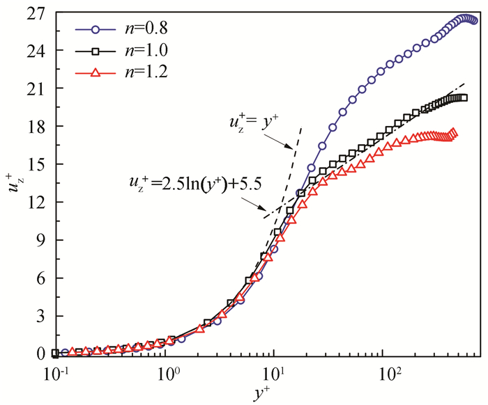
Fig. 3 displays the trends of mean axial velocity with the power-law indexes of 0.8, 1.0, and 1.2, respectively. Obviously, the log-region expands with the decrease of the power-law index, while the normalized velocity profiles comply with the linear law in 0 ≤ y+ < 5. In the turbulent core region, the velocity distribution meets the following logarithmic function at n=1:
| $ {u^ + } = 2.5\ {\rm{ln}}({y^ + }) + 5.5\left( {n = 1} \right) $ | (9) |
|
Fig.3 Effect of power-law index on turbulent axial velocity profiles |
When n=0.8 and 1.2, they deviate from this function, especially the deviation at n=0.8 is more obvious. Such variation tendency agrees with the simulation results of Rudman et al.[6] by DNS, which also shows more obvious deviation at n < 1. It is therefore suggested that the shear-thinning fluid exhibits remarkably non-Newtonian character.
2.2 Friction FactorIn this section, the simulation friction factor by LES was compared with the results from empirical formulae. The fanning friction factor refers to a local parameter used to calculate the continuum mechanics; it is also a dimensionless group. The formula represents the ratio of local shear stress to local kinetic energy density:
| $ f = {\tau _w}/(\rho u_{_b}^2/2) $ | (10) |
where the mean wall shear stress is
In general, the friction factor at n≤1 is obtained from empirical formulae by Dodge and Meetzner[21] correlation and Gomes correlation coefficient[17], which are as follows:
| $ \begin{array}{c} {f_{{\rm{DM}}}} = a/{\rm{Re}}_{{\rm{MR}}}^b\\ a = 0.0665 + 0.01175n\\ b = 0.365{\rm{ - }}0.177n + 0.062{n^2}\\ {f_G} = 0.110{n^{0.616}}{\rm{R}}{{\rm{e}}^{{\rm{ - }}0.287}} \end{array} $ |
The calculated friction factors are listed in Table 2. The friction factor decreases with the decrease of the power-law index in fully developed turbulence. It is consistent with experimental observations by Dodge and Metzner[21], in which shear-thinning behavior is supposed to be the main cause of the decrease in the friction factor at a specific ReMR[21]. The errors between LES and the two empirical formulae are 3.51% and 6% at n=1, while they are 4.1% and 3.7% for n=0.8. Similar errors have also appeared in Refs. [22-23], where the errors are 5%-8% and 10%, higher than Dodge and Meetzner correlation.
| Table 2 Friction factor |
2.3 Mean Normalized Viscosity
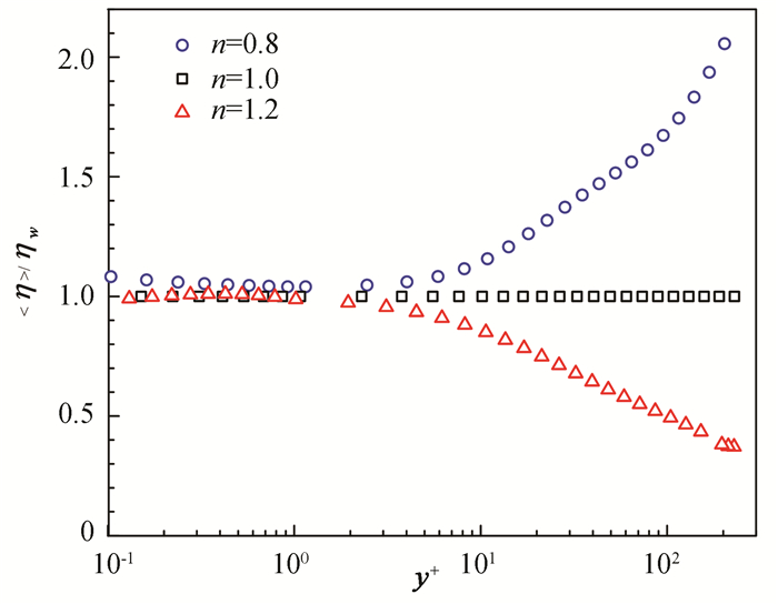
The mean normalized viscosity 〈η〉/ηw refers to the radio of the mean viscosity to the mean wall viscosity. Fig. 4 presents the relation between the normalized apparent viscosity and the dimensionless distance (y+). In the near-wall region (y+ > 5), the apparent viscosity keeps a constant. The viscosity of shear-thinning fluid increases with the increase of y+, while the shear-thickening fluid shows the reverse trend in log-region. The viscosity of Newtonian fluid remains unchanged. It is also observed that the deviation of the shear-thinning fluid from Newtonian fluid is larger than that of the shear-thickening fluid, complying with results by Gnambode et al. [17]
|
Fig.4 Mean viscosity profiles as a function of different power-law indexes |
Fig. 5 depicts the variation of mean normalized viscosity as the mean normalized shear rate

|
Fig.5 Mean normalized viscosity as a function of mean normalized shear rate with different power-law indexes |
2.4 RMS of Turbulent Fluctuation
Fig. 6 shows RMS of axial and radial velocity fluctuation urms+ against results based on DNS by Khoury et al.[18] The superscript (+) indicates normalization of the friction velocity with the wall uτ=(τw/ρ)1/2, where τw denotes the wall shear stress. In the figure, the turbulent intensity increases to the maximum value and then decreases from the wall to the center. For the axial velocity fluctuation uz, rms+, the maximum value is about 2.8 at y+ > 15. However, the radial velocity fluctuation reaches a maximum at a position slightly away from the wall. The RMS of the velocity fluctuation is consistent with the results based on DNS by Khoury et al.[18]

|
Fig.6 RMS of axial and radial velocity fluctuations against results based on DNS |
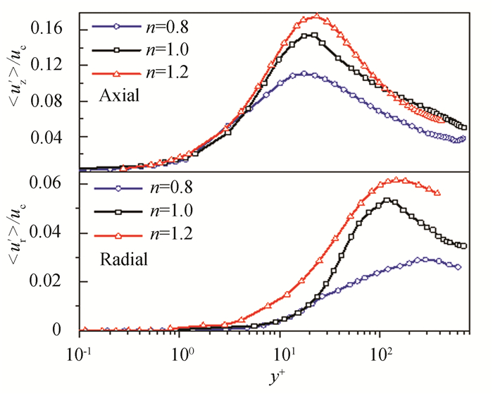
Fig. 7 describes the RMS of fluctuating axial velocity and radial velocity with different power-law indexes. As the power-law index increases, the maximum value of the RMS of axial velocity fluctuation increases, and gradually deviates from the wall toward the center. The value moves from y+ ≈ 17.69 at n=0.8 to y+ ≈ 23.63 at n=1.2. Near the wall, the apparent viscosity increases with the increase of the power-law index, whereas it tends to decrease far from the wall. Thus, the shear-thinning fluid reaches a maximum closer to the wall than shear-thickening fluid.
|
Fig.7 RMS of axial and radial velocity fluctuations with different power-law indexes |
Compared with axial velocity, the radial velocity is smaller in fluctuation, and their maximum values appear nearer to the center. For y+ > 20, the turbulent intensity decreases with the decrease of the power-law index, indicating that the mean apparent viscosity of the region increases. For shear-thinning fluid, the increment in mean viscosity near the center leads to larger and weaker axial vortices, thus reducing wall resistance. For n > 1, the mean viscosity at the center is smaller, thereby reducing energy dissipation and narrowing the turbulence structures in the region.
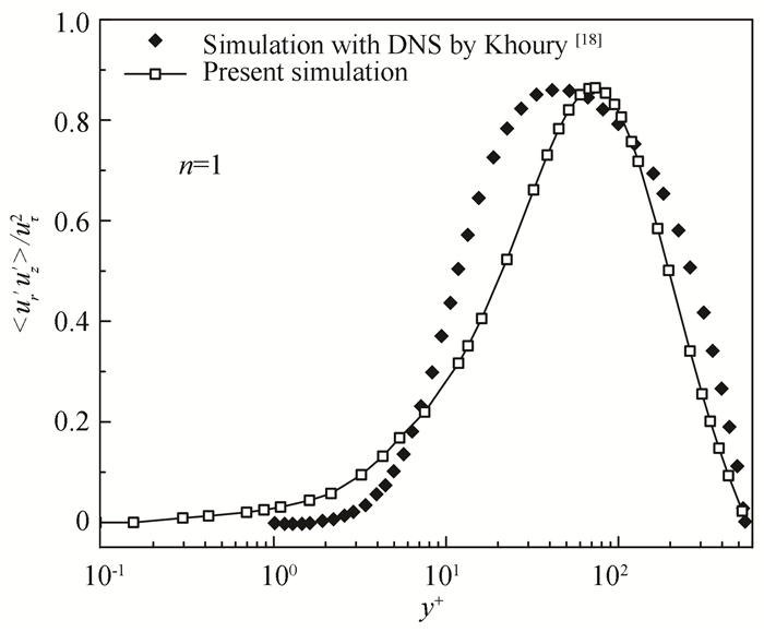
2.5 Reynolds StressFig. 8 presents a comparison of Reynolds stress of Newtonian fluid by LES with the direct numerical simulation results by Khoury et al.[18] The Reynolds stress is low near the wall. With the increase of y+, the value progressively rises and then decreases gradually after reaching the peak near y+=40. The reason for this discrepancy might be that the current Reynolds number (Reτ=581) is slightly different from the DNS (Reτ=550).
|
Fig.8 Reynolds shear stress compared to DNS for Newtonian fluid |
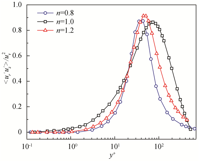
The Reynolds stresses of different power-law indexes are plotted in Fig. 9. The variation of Reynolds shear stress with the power-law index is similar to axial turbulence intensity. The variation tendency in Reynolds shear stress is similar to the axial turbulence intensity with the power-law index. With the decrease of the power-law index, the peak value declines. The main reason for this phenomenon is that with the decrease of the power-law index, its apparent viscosity is enhanced, resulting in a decline in the momentum from the center to the wall.
|
Fig.9 Effect of power-law index on Reynolds shear stress |
2.6 Skewness and Flatness
The skewness indicates the asymmetry of the probability density function of fluctuating velocity. The non-zero skewness denotes the skewness or asymmetry of the PDF. It can be expressed as
| $ S(u_i') = \langle u_i^{'3}\rangle /{\left\langle {u_i^{'2}} \right\rangle ^{\frac{3}{2}}} $ | (11) |
The flatness represents the intermittence of random variables, revealing that large-valued random variables occur at higher frequencies, compared with normal distribution. It is expressed as
| $ F(u_i') = \left\langle {u_{_i}^{'4}} \right\rangle /{\left\langle {u_{_i}^{'2}} \right\rangle ^2} $ | (12) |
In general, the flatness of intermittent random variables is greater than that of Gauss distribution. The flatness of Gauss distribution is 3, hence random variables with a flatness greater than 3 are considered intermittent.
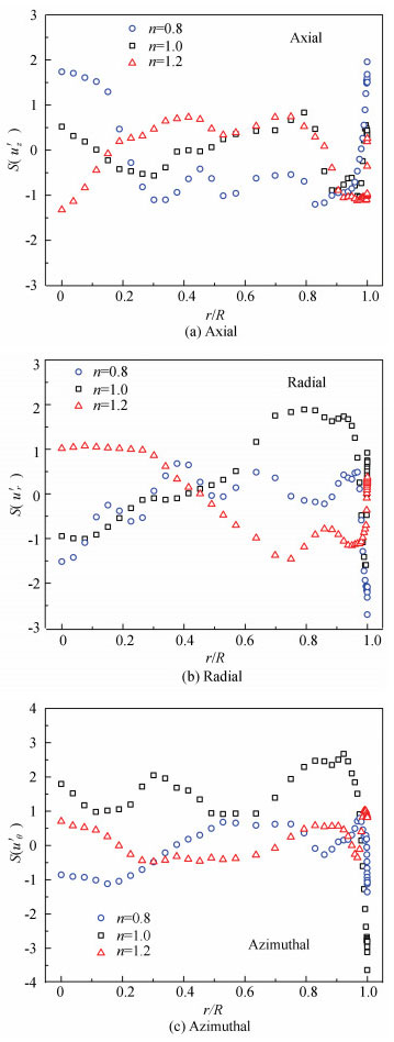
The distributions of the skewness and flatness coefficients of the velocity fluctuation are plotted in Figs. 10-11. It is well known that the distribution of turbulent fluctuation is distinct from normal distribution, whose skewness and flatness of normal distribution are 0 and 3, respectively. The turbulent fluctuation is not an absolutely random flow process, but it has inherent correlations. As shown in Fig. 10, in the near-wall area, the absolute value of three skewness coefficient increases quickly and deviates obviously from the Gauss distribution with the decrease of the power-law index, indicating that the asymmetry of fluctuating velocity at the wall increases the decreasing of power-law index. However, in the region away from the wall, there are positive and negative flow pulsations regardless of different power-law indexes, approaching to the Gauss distribution. These volatilities have essential association with the near-wall bursting process. Moreover, the skewness coefficient of the azimuthal velocity fluctuation approaches to the Gaussian value towards the core region more as power-law index increases, as shown in Fig. 10(c).
|
Fig.10 Skewness of the velocity fluctuations |
|
Fig.11 Flatness of the velocity fluctuations |
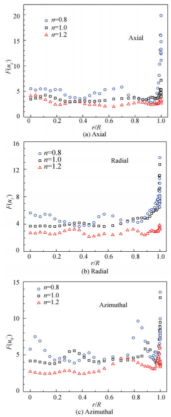
Back to Fig. 11, the near-wall flatness coefficient is sensitive to power-law index. As revealed from the figure, with the decrease of the power-law index, the flatness coefficient increases rapidly, indicating that the velocity fluctuation near the wall is more intermittent. Accordingly, the velocity fluctuations for all components near the wall are more obvious than those in the center of the pipe. Away from the wall, the flatness coefficient is relatively small, and the flatness coefficient is close to 3 at n > 1, which means it tends to be normal flow.
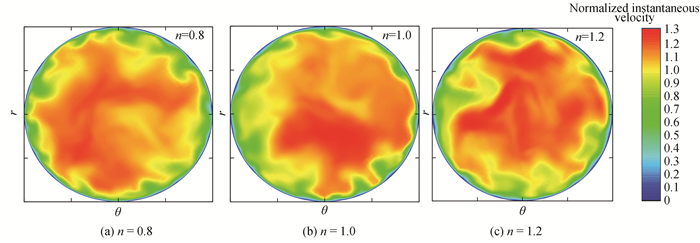
2.7 Flow PicturesThe normalized instantaneous axial velocity and viscosity contours with different power-law indexes are depicted in Figs. 12-13, where the instantaneous axial velocity is normalized by bulk velocity ub, and the instantaneous viscosity is normalized by maximum viscosity. The figures show that the increase of power-law index leads to the appearance of more fine scale structures, while the viscosity profiles of the three fluids are inconsistent, as shown in Fig. 13. In the whole cross-section, the shear rate near the wall is the largest, the near-wall viscosity of shear-thinning fluid is lower than that of the pipe center, while the phenomenon of shear-thickening fluid is the opposite. Generally speaking, the viscosity directly affects the fluidity of fluid. Therefore, the velocity distribution of shear-thickening fluid near the core is more uneven than that of shear-thinning fluid, and the velocity of shear-thinning fluid near the wall varies more sharply than shear-thickening fluid. This is consistent with the rule that the turbulence intensity is enhanced with the increase of the power-law index, indicating that the turbulence is more developed as power-law index increases.
|
Fig.12 Contours of instantaneous axial velocity normalized by the bulk velocity |

|
Fig.13 Contours of instantaneous viscosity normalized by the maximum viscosity |
3 Conclusions
The dynamic subgrid-scale model of LES was used to study the effects of the power-law index on fully developed turbulence at ReMR ≈ 20000. The current prediction is in good agreement with the results reported by Gnambode et al.[17] and Khoury et al.[18] In the full development of turbulence, the axial velocity profile satisfied the linear law (u+ = y+) in y+ < 5 and the logarithmic law in log-region. As for different power-law indexes at the same Reynolds number, the mean axial velocity deviated from the Newtonian in varying degrees. With the decrease of the power-law index, the mean normalized apparent viscosity increased in log-region, and the departure degree of the shear-thinning fluid was larger than that of the shear-thickening fluid. The peak values of RMS of velocity fluctuation and Reynolds stress decreased as the apparent viscosity increased in the log-region. The skewness and flatness coefficients of the axial velocity fluctuation increased in the near-wall region, indicating a more significant asymmetry and intermittency behavior with the decrease of power-law index. The contours of the normalized instantaneous axial velocity and viscosity demonstrate that the turbulence intensity increased with the rise of the power-law index. In summary, dynamic subgrid-scale stress model can reproduce detailed characteristics of non-Newtonian fluids flow and reduce the computational cost, revealing that the dynamic subgrid-scale model may be a powerful tool to turbulence in a circular pipe at a higher Reynolds number.
| [1] |
Escudier M P, Presti F. Pipe flow of a thixotropic liquid. Journal of Non-Newtonian Fluid Mechanics, 1996, 62(2-3): 291-306. DOI:10.1016/0377-0257(96)01417-6 (  0) 0) |
| [2] |
Sureshkumar R, Beris A N, Handler R A. Direct numerical simulation of the turbulent channel flow of a polymer solution. Physics of Fluids, 1997, 9(3): 743-755. DOI:10.1063/1.869229 (  0) 0) |
| [3] |
Guillou S, Makhloufi R. Effect of a shear-thickening rheological behaviour on the friction coefficient in a plane channel flow: a study by direct numerical simulation. Journal of Non-Newtonian Fluid Mechanics, 2007, 144: 73-86. DOI:10.1016/j.jnnfm.2007.03.008 (  0) 0) |
| [4] |
Wang Y, Sun S Y, Gong L, et al. A globally mass-conservative method for dual-continuum gas reservoir simulation. Journal of Natural Gas Science and Engineering, 2018, 53: 301-316. DOI:10.1016/j.jngse.2018.03.009 (  0) 0) |
| [5] |
Wang Y, Wang Y, Cheng Z. Direct numerical simulation of gas-liquid drag-reducing cavity flow by the VOSET method. Polymers, 2019, 11(4): 596-612. DOI:10.3390/polym11040596 (  0) 0) |
| [6] |
Rudman M, Blackburn H M, Graham L J W., et al. Turbulent pipe flow of shear-thinning fluids. Journal of Non-Newtonian Fluid Mechanics, 2004, 118(1): 33-48. DOI:10.1016/j.jnnfm.2004.02.006 (  0) 0) |
| [7] |
Pinho F T, Whitelaw J H. Flow of non-newtonian fluids in a pipe. Journal of Non-Newtonian Fluid Mechanics, 1990, 34(2): 129-144. DOI:10.1016/0377-0257(90)80015-R (  0) 0) |
| [8] |
Bogue D C, Metzner A B. Velocity profiles in turbulent pipe flow: Newtonian and non-Newtonian fluids. Industrial & Engineering Chemistry Fundamentals, 1963, 2(2): 143-149. DOI:10.1021/i160006a010 (  0) 0) |
| [9] |
Rudman M, Graham L J, Blackburn H M. Non-Newtonian turbulent and transitional pipe flow. Proceedings of the 15th International Conference on Hydrotransport incorporating the 11th International Symposium of Freight Pipelines. Bedfordshire, U.K. : BHR Group, 2002. 271-286.
(  0) 0) |
| [10] |
Wang Y. Reynolds stress model for viscoelastic drag-reducing flow induced by polymer solution. Polymers, 2019, 11(10): 1659-1669. DOI:10.3390/polym11101659 (  0) 0) |
| [11] |
Cui G X, Xu C X, Zhang Z S. Progress in large eddy simulation of turbulent flows. Acta Aerodynamica Sinica, 2004, 22(2): 121-129. (  0) 0) |
| [12] |
Ohta T, Miyashita M. DNS and LES with an extended Smagorinsky model for wall turbulence in non-Newtonian viscous fluids. Journal of Non-Newtonian Fluid Mechanics, 2014, 206: 29-39. DOI:10.1016/j.jnnfm.2014.02.003 (  0) 0) |
| [13] |
Dairay T, Lamballais E, Benhamadouche S. Mesh node distribution in terms of wall distance for large-eddy simulation of wall-bounded flows. Flow, Turbulence and Combustion, 2018, 100: 617-626. DOI:10.1007/s10494-017-9863-5 (  0) 0) |
| [14] |
Cheng W, Samtaney R. Power-law versus log-law in wall-bounded turbulence: a large-eddy simulation perspective. Physics of Fluids, 2014, 26(1): 011703-1-011703-7. DOI:10.1063/1.4862919 (  0) 0) |
| [15] |
Thais L, Tejada-Martinez A E, Gatski T B. Temporal large eddy simulations of turbulent viscoelastic drag reduction flows. Physics of Fluids, 2010, 22: 013103-1-013103-13. DOI:10.1063/1.3294574 (  0) 0) |
| [16] |
Molla M M, Paul M C. LhhhES of non-Newtonian physiological blood flow in a model of arterial stenosis. Medical Engineering & Physics, 2012, 34(8): 1079-1087. DOI:10.1016/j.medengphy.2011.11.013 (  0) 0) |
| [17] |
Gnambode P S, Orlandi P, Ould-Rouiss M, et al. Large-Eddy simulation of turbulent pipe flow of power-law fluids. International Journal of Heat & Fluid Flow, 2015, 54: 196-210. DOI:10.1016/j.ijheatfluidflow.2015.05.004 (  0) 0) |
| [18] |
Khoury G K, Schlatter P, Noorani A, et al. Direct numerical simulation of turbulent pipe flow at moderately high Reynolds Numbers. Flow, Turbulence and Combustion, 2013, 91(3): 475-495. (  0) 0) |
| [19] |
Germano M, Piomelli U, Moin P, et al. A dynamic subgrid-scale eddy viscosity model. Physics of Fluids A, 1991, 3(7): 1760-1765. DOI:10.1063/1.857955 (  0) 0) |
| [20] |
Lilly D K. A proposed modification of the Germano subgrid-scale closure method. Physics of Fluids A: Fluid Dynamics, 1992, 4(3): 633-635. DOI:10.1063/1.858280 (  0) 0) |
| [21] |
Dodge D W, Metzner A B. Turbulent flow of non-Newtonian systems. AIChE Journal, 1959, 5(2): 189-204. DOI:10.1002/aic.690050214 (  0) 0) |
| [22] |
Gavrilov A A, Rudyak V Y. Reynolds-averaged modeling of turbulent flows of power-law fluids. Journal of Non-Newtonian Fluid Mechanics, 2016, 227: 45-55. DOI:10.1016/j.jnnfm.2015.11.006 (  0) 0) |
| [23] |
Rudman M, Blackburn H M. Direct numerical simulation of turbulent non-Newtonian flow using a spectral element method. Applied Mathematical Modelling, 2006, 30(11): 1229-1248. DOI:10.1016/j.apm.2006.03.005 (  0) 0) |
 2021, Vol. 28


