The general unconstrained optimization problem is considered in this study. Its form is as follows:
| $ \min f(\boldsymbol{x}), \boldsymbol{x} \in {\bf{R}}^{n} $ | (1) |
where f: R n→ R is the objective function. CG method is one of the most important methods for solving the large-scale unconstrained optimization problem (1). Let αk be a stepsize, then the iterations satisfy the iterative format:
| $ \boldsymbol{x}_{k+1}=\boldsymbol{x}_{k}+\alpha_{k} \boldsymbol{d}_{k} $ | (2) |
where dk is search direction and denoted by
| $ \boldsymbol{d}_{k+1}= \begin{cases}-\boldsymbol{g}_{k+1}+{\beta}_{k} \boldsymbol{d}_{k}, & k>0 \\ -\boldsymbol{g}_{k+1}, & k=0\end{cases} $ | (3) |
where βk∈R is the CG parameter and gk+1= ▽f(xk+1).
When the functions are general nonlinear, various selections of βk result in different CG methods. Some of the great name options for βk are FR, HS, PRP, DY, and HZ formula[1-5], and are given by
| $ \beta_{k}^{\mathrm{FR}}=\frac{\left\|\boldsymbol{g}_{k+1}\right\|^{2}}{\left\|\boldsymbol{g}_{k}\right\|^{2}}, {\beta}_{k}^{\mathrm{HS}}=\frac{\boldsymbol{g}_{k+1}^{\mathrm{T}} \boldsymbol{y}_{k}}{\boldsymbol{d}_{k}^{\mathrm{T}} \boldsymbol{y}_{k}} $ |
| $ \beta_{k}^{\mathrm{PRP}} =\frac{\boldsymbol{g}_{k+1}^{\mathrm{T}} \boldsymbol{y}_{k}}{\left\|\boldsymbol{g}_{k}\right\|^{2}}, {\beta}_{k}^{\mathrm{DY}}=\frac{\left\|\boldsymbol{g}_{k+1}\right\|^{2}}{\boldsymbol{d}_{k}^{\mathrm{T}} \boldsymbol{y}_{k}} $ |
| $ {\beta}_{k}^{\mathrm{HZ}} =\frac{1}{\boldsymbol{d}_{k}^{\mathrm{T}} \boldsymbol{y}_{k}}\left(\boldsymbol{y}_{k}-2 \boldsymbol{d}_{k} \frac{\left\|\boldsymbol{y}_{k}\right\|^{2}}{\boldsymbol{d}_{k}^{\mathrm{T}} \boldsymbol{y}_{k}}\right)^{\mathrm{T}} \boldsymbol{g}_{k+1} $ |
where ‖.‖ points to the Euclidean norm and yk=gk+1-gk. In recent years, other effective CG methods have different views[6-8].
With the increasing scale of optimization problems, the subspace technique is favored by more and more researchers. Subspace procedures are a kind of extremely effective numerical procedures to solve wide-ranging optimization issues instead of wide-ranging subproblems, as it is not necessary to solve wide-ranging subproblems in per iteration [9]. In 1995, Yuan and Stoer[10] first stated the subspace minimization CG (SMCG) algorithm, in which the search direction was calculated by minimizing a quadratic estimated model on Ωk+1={sk, gk+1}, i.e.:
| $ \boldsymbol{d}=v \boldsymbol{s}_{k}+\mu \boldsymbol{g}_{k+1} $ | (4) |
where sk=xk+1-xk and μ, v are parameters. They considered the following problem:
| $ \min \limits_{d \in \Omega_{k+1}} m_{k+1}(\boldsymbol{d})=\boldsymbol{g}_{k+1}^{\mathrm{T}} \boldsymbol{d}+\frac{1}{2} \boldsymbol{d}^{\mathrm{T}} \boldsymbol{B}_{k+1} \boldsymbol{d} $ | (5) |
where Bk+1 is a rough calculation to Hessian matrix. SMCG method is an extension of the classical CG method and is a kind of efficient optimization method, which has attracted the attention of some researchers. Because a three-dimensional subspace contains more information of the iteration point than a two-dimensional one, inspired by SMCG, Li et al.[11] extended SMCG to three-dimensional (Ωk+1={gk+1, sk, sk-1 }) subspace minimization conjugate gradient method (SMCG_NLS), and numerical comparisons showed that the proposed method worked effectively.
Generally, a quadratic mold may well estimate f(x) in a smaller neighborhood of the minimizer, so the iterative procedures are usually on account of this model. However, when the objective function has high non-linearity, a quadratic model may not approximate it very well, since iteration dot is far from the minimizer. To address the drawback, some cubic regularization algorithms for unconstrained optimization are getting increasingly more attention[12-13]. The idea is to incorporate a local quadratic approximation of the objective function with a cubic regularization term and then globally minimize it at each iteration. The cubic regularization was first introduced by Griewank[14] and was later considered by many authors with global convergence and complexity analysis[15]. In fact, the cubic regularization algorithm needs to carry out multiple iterative solution exploratory steps in the subspace, which makes the solution of the subproblem more complex and requires a lot of calculation and storage space. The solution of the problem is the most important and the most cost-consuming part of the algorithm. Therefore, how to construct an approximate model closer to the objective function and how to efficiently solve the subproblem of the algorithm are the core of the challenge.
In this study, a new three-term SMCG method inspired by SMCG_NLS is raised on account of a cubic regularization model with a special scaled norm (compared with RC, when the l2- norm is used to define the regularization term in the subproblem, the dominant computational cost of the resulting algorithm is mainly the cost of successful iterations, as the unsuccessful ones are inexpensive). Generally, when the objective function approaches a quadratic function, the performance of a quadratic model is better, so the quadratic model is chosen. Therefore, this study considers the dynamic selection of the appropriate approximate model, i.e., a quadratic model or a cubic regular model, further proposes a new algorithm, and analyzes the convergence of the new algorithm. Finally, numerical experiments verify the effectiveness of the algorithm.
1 Form and Solution of the Cubic Regularized SubproblemIn this section, the form of the cubic regularized subproblem is briefly introduced by using a special scaled norm and the solution of the problem is provided.
The ordinary form of the cubic regularized subproblem is given by
| $ \min \limits_{\boldsymbol{x} \in {\bf{R}}^{n}} \mathrm{~g}(\boldsymbol{x})=\boldsymbol{c}^{\mathrm{T}} \boldsymbol{x}+\frac{1}{2} \boldsymbol{x}^{\mathrm{T}} \boldsymbol{H} \boldsymbol{x}+\frac{\sigma}{3}\|\boldsymbol{x}\|^{3} $ | (6) |
where c∈ Rn, σ>0, and H∈ Rn×n is a symmetric positive definite matrix.
From Theorem 3.1 of Ref. [15], it is known the point x* is a global minimizer of Eq.(6) if and only if
| $ \left(\boldsymbol{H}+\sigma\left\|\boldsymbol{x}^{*}\right\| \boldsymbol{I}\right) \boldsymbol{x}^{*}=-\boldsymbol{c} $ | (7) |
where I is the unit array. If H+ σ ‖x*‖ I is positive definite, x* is unique.
Subsequently, another form of the cubic regularized subproblem with a special scaled norm is given:
| $ \min \limits_{\boldsymbol{x} \in {\bf{R}}^{n}} g(\boldsymbol{x})=\boldsymbol{c}^{\mathrm{T}} x+\frac{1}{2} \boldsymbol{x}^{\mathrm{T}} \boldsymbol{H} \boldsymbol{x}+\frac{\sigma}{3}\|\boldsymbol{x}\|_{H}^{3} $ | (8) |
where
By setting
| $ \min \limits_{\hat{\boldsymbol{y}} \in {\bf{R}}^{n}} g(\hat{\boldsymbol{y}})=\left(\boldsymbol{H}^{-\frac{1}{2}} \boldsymbol{c}\right)^{\mathrm{T}} \hat{\boldsymbol{y}}+\frac{1}{2} \hat{\boldsymbol{y}}^{\mathrm{T}} \boldsymbol{I} \hat{\boldsymbol{y}}+\frac{\sigma}{3}\|\hat{\boldsymbol{y}}\|^{3} $ | (9) |
According to Eq.(7), the point
| $ \left(\boldsymbol{I}+\boldsymbol{\sigma}\left\|\hat{\boldsymbol{y}}^{*}\right\| \boldsymbol{I}\right) \hat{\boldsymbol{y}}^{*}=-\boldsymbol{H}^{-\frac{1}{2}} \boldsymbol{c} $ | (10) |
Let V ∈ Rn×n be an orthogonal matrix, so VTV = I. Now the vector a ∈ Rn can be introduced, which yields
Denote z=‖
| $ (1+\sigma \boldsymbol{z}) \boldsymbol{I} \boldsymbol{a}=-\boldsymbol{\beta} $ |
where β = VT(
The last expression can be equivalently written as
| $ a_{i}=\frac{-\beta_{i}}{1+\sigma z}, i=1,2, \cdots, n $ |
where ai and βi are the components of vectors a and β, respectively.
According to z=‖
| $ \boldsymbol{z}^{2}=\hat{\boldsymbol{y}}^{\mathrm{T}} \hat{\boldsymbol{y}}=\boldsymbol{a}^{\mathrm{T}} \boldsymbol{a}=\sum\limits_{i=1}^{n} \frac{-\beta_{i}^{2}}{(1+\sigma \boldsymbol{z})^{2}}=\frac{\boldsymbol{c}^{\mathrm{T}} \boldsymbol{H}^{-1} \boldsymbol{c}}{(1+\sigma \boldsymbol{z})^{2}} $ | (11) |
Based on the above derivation and analysis, the following corollary is obtained:
Corollary 1.1 The point
| $ \sigma \boldsymbol{z}^{2}+\boldsymbol{z}-\sqrt{\boldsymbol{c}^{\mathrm{T}} \boldsymbol{H}^{-1} \boldsymbol{c}}=0 $ |
Proof : According to Eq.(10), I +σ‖
In this section, the search direction is deduced by minimizing a cubic regularization model or a quadratic estimation of f(x) on Ωk+1={sk, gk+1, sk-1}. A generalized Wolfe line search is also developed. For the other parts, it is supposed that skTyk>0, which is ensured by ▽f(xk+αk dk)Tdk≥σ▽f(xk)Tdk.
2.1 Deduction of the New Search DirectionIn this study, the following was defined at each iteration:
| $ t_{k}=\left|\frac{2\left(f_{k}-f_{k+1}+\boldsymbol{g}_{k+1}^{\mathrm{T}} \boldsymbol{s}_{k}\right)}{\boldsymbol{s}_{k}^{\mathrm{T}} \boldsymbol{y}_{k}}-1\right| $ |
According to Ref. [16], tk is a quantity which displays how close the objective function is to a quadratic function on the line segment between the current iteration point and the previous iteration point. If the condition
| $ t_{k} \leqslant \omega_{1} \text { or }\left(t_{k} \leqslant \omega_{2} \text { and } t_{k-1} \leqslant \omega_{2}\right) $ | (12) |
holds, where 0 ω1≤ω2, it is believed that objective function is extremely close to a quadratic on the line segment between xk-1 and xk, then a quadratic estimation model is considered. Otherwise, the cubic regularization model might be more suitable because they basically improve the gradient evaluation complexity and worst-case iteration [17]. So dk is gained by minimizing a cubic regularization mold or a quadratic mold in the three-dimensional subspace.
The following regularization model of f(x) was considered:
| $ \min \limits_{d \in \Omega_{k+1}} m_{k+1}(\boldsymbol{d})=\boldsymbol{d}^{\mathrm{T}} \boldsymbol{g}_{k+1}+\frac{1}{2} \boldsymbol{d}^{\mathrm{T}} \boldsymbol{H}_{k+1} \boldsymbol{d}+\frac{1}{3} \sigma_{k+1}\|\boldsymbol{d}\|_{\boldsymbol{H}_{k+1}}^{3} $ | (13) |
where σk+1 is a dynamic non-negative regularization parameter, Hk+1 is a positive and symmetric definite matrix, satisfying the equation Hk+1sk= yk and Ωk+1=span{gk+1, sk, sk-1}.
It can be found that mk+1(d) has the following properties: if σk+1=0, Eq.(13) produces a quadratic approximate model. So let σk+1=0 when condition Eq.(12) holds; otherwise, σk+1 is obtained by interpolation function. Obviously, the dimension of Ωk+1 maybe 3, 2, or 1. The search direction are exported from the following three situations.
Situation 1: dim (Ωk+1)=3. In this situation, the search direction dk+1 may be given by
| $ \boldsymbol{d}_{k+1}=\mu \boldsymbol{g}_{k+1}+\nu \boldsymbol{s}_{k}+\tau \boldsymbol{s}_{k-1} $ | (14) |
where μ, v, and τ are coefficients to be determined.
By substituting Eq.(14) into Eq.(13), the following cubic regularized subproblem about μ, v, and τ is obtained:
| $ \begin{array}{l} \min \limits_{(\mu, \nu, \tau) \in \mathrm{R}}\left(\begin{array}{l} \left\|\boldsymbol{g}_{k+1}\right\|^{2} \\ \boldsymbol{g}_{k+1}^{\mathrm{T}} \boldsymbol{s}_{k} \\ \boldsymbol{g}_{k+1}^{\mathrm{T}} \boldsymbol{s}_{k-1} \end{array}\right)^{\mathrm{T}}\left(\begin{array}{l} \mu \\ \nu \\ {\tau} \end{array}\right)+\frac{1}{2}\left(\begin{array}{l} \mu \\ \nu \\ \tau \end{array}\right)^{\mathrm{T}} \boldsymbol{B}_{k+1}\left(\begin{array}{l} \mu \\ \nu \\ {\tau} \end{array}\right)+ \\ \;\;\;\;\;\;\;\;\;\;\frac{{\sigma}_{k+1}}{3}\left\|\left(\begin{array}{l} \mu \\ \nu \\ {\tau} \end{array}\right)\right\|_{{B}_{k+1}}^{3} \end{array} $ | (15) |
where
| $ {\rho}_{k} \approx \boldsymbol{g}_{k+1}^{\mathrm{T}} \boldsymbol{H}_{k+1} \boldsymbol{g}_{k+1} $ |
| $ \boldsymbol{B}_{k+1}=\left(\begin{array}{lcc} {\rho}_{k} & \boldsymbol{g}_{k+1}^{\mathrm{T}} \boldsymbol{y}_{k} & \boldsymbol{g}_{k+1}^{\mathrm{T}} \boldsymbol{y}_{k-1} \\ \boldsymbol{g}_{k+1}^{\mathrm{T}} \boldsymbol{y}_{k} & \boldsymbol{s}_{k}^{\mathrm{T}} \boldsymbol{y}_{k} & \boldsymbol{s}_{k-1}^{\mathrm{T}} \boldsymbol{y}_{k} \\ \boldsymbol{g}_{k+1}^{\mathrm{T}} \boldsymbol{y}_{k-1} & \boldsymbol{s}_{k-1}^{\mathrm{T}} \boldsymbol{y}_{k} & \boldsymbol{s}_{k-1}^{\mathrm{T}} \boldsymbol{y}_{k-1} \end{array}\right) $ |
It can be easily found that the problem Eq.(15) is analogous to Eq.(8) in Ref. [11] with only one more regular term. Obviously, if the matrix Bk+1 in Eq.(15) is positive definite, the unique solution of (15) can be obtained. To estimate gk+1THk+1gk+1 properly and keep Bk+1 positive definite, ρk is defined as follows:
| $ \rho_{k}=\frac{3}{2} \max \left\{n_{k}, K\right\} $ | (16) |
where
| $ n_{k}=\left(\frac{\left(\boldsymbol{g}_{k+1}^{\mathrm{T}} \boldsymbol{y}_{k-1}\right)^{2}}{\boldsymbol{s}_{k-1}^{\mathrm{T}} \boldsymbol{y}_{\mathrm{k}-1}}+\frac{\left(\boldsymbol{g}_{k+1}^{\mathrm{T}} \boldsymbol{y}_{k}\right)^{2}}{\boldsymbol{s}_{k}^{\mathrm{T}} \boldsymbol{y}_{k}}-\frac{2 \boldsymbol{g}_{k+1}^{\mathrm{T}} \boldsymbol{y}_{k} \boldsymbol{g}_{k+1}^{\mathrm{T}} \boldsymbol{y}_{k-1} \boldsymbol{s}_{k-1}^{\mathrm{T}} \boldsymbol{y}_{k}}{\boldsymbol{s}_{k-1}^{\mathrm{T}} \boldsymbol{y}_{k-1} \boldsymbol{s}_{k}^{\mathrm{T}} \boldsymbol{y}_{k}}\right) / m_{k} $ |
| $ K=K_{1}\left\|\boldsymbol{g}_{k+1}\right\|^{2}, K_{1}=\max \left\{\frac{\left\|\boldsymbol{y}_{k}\right\|^{2}}{\boldsymbol{s}_{k}^{\mathrm{T}} \boldsymbol{y}_{k}}, \frac{\left\|\boldsymbol{y}_{k-1}\right\|^{2}}{\boldsymbol{s}_{k-1}^{\mathrm{T}} \boldsymbol{y}_{k-1}}\right\} $ |
| $ m_{k}=1.0-\left(\boldsymbol{s}_{k-1}^{\mathrm{T}} \boldsymbol{y}_{k}\right)^{2} /\left(\boldsymbol{s}_{k-1}^{\mathrm{T}} \boldsymbol{y}_{k-1} \boldsymbol{s}_{k}^{\mathrm{T}} \boldsymbol{y}_{k}\right) $ |
which can be seen in Ref. [11].
From Corollary 1.1, the unique solution to Eq.(15) can be obtained:
| $ \left(\begin{array}{l} \mu_{k} \\ \nu_{k} \\ \tau_{k} \end{array}\right)=\frac{-1}{1+\sigma_{k+1} \boldsymbol{z}^{*}} \boldsymbol{B}_{k+1}^{-1}\left(\begin{array}{c} \left\|\boldsymbol{g}_{k+1}\right\|^{2} \\ \boldsymbol{g}_{k+1}^{\mathrm{T}} \boldsymbol{s}_{k} \\ \boldsymbol{g}_{k+1}^{\mathrm{T}} \boldsymbol{s}_{k-1} \end{array}\right) $ | (17) |
So dk+1 can be calculated by Eq.(17) and Eq.(14) under the following conditions:
| $ \rho_{0} \leqslant m_{k}, \xi_{3} \leqslant \frac{\left\|\boldsymbol{s}_{k}\right\|^{2}}{\left\|\boldsymbol{g}_{k+1}\right\|^{2}} $ | (18) |
| $ \xi_{1} \leqslant \frac{\boldsymbol{s}_{k}^{\mathrm{T}} \boldsymbol{y}_{k}}{\left\|\boldsymbol{s}_{k}\right\|^{2}} \leqslant \frac{\left\|\boldsymbol{y}_{k}\right\|^{2}}{\boldsymbol{s}_{k}^{\mathrm{T}} \boldsymbol{y}_{k}} \leqslant \xi_{2} $ | (19) |
and
| $ \xi_{1} \leqslant \frac{\boldsymbol{s}_{k-1}^{\mathrm{T}} \boldsymbol{y}_{k-1}}{\left\|\boldsymbol{s}_{k-1}\right\|^{2}} \leqslant \frac{\left\|\boldsymbol{y}_{k-1}\right\|^{2}}{\boldsymbol{s}_{k-1}^{\mathrm{T}} \boldsymbol{y}_{k-1}} \leqslant \xi_{2} $ | (20) |
where ρ0∈(0, 1) and ξ1, ξ2, ξ3>0. It can be found that the eigenvalues of the submatri
Remark 1: Bk+1 in Eq.(15) is different from Bk+1 in Eq.(5). In model Eq.(13), Hk+1 was used to represent the rough calculation of Hessian matrix.
Situation 2: dim(Ωk+1)=2. If only condition (19) successfully holds, Ωk+1=span {gk+1, sk} is considered.dk+1 may be described by
| $ \boldsymbol{d}_{k+1}=\mu \boldsymbol{g}_{k+1}+v \boldsymbol{s}_{k} $ | (21) |
where μ and v are parameters to be determined. Substituting Eq.(21) into Eq.(13), the corresponding problem Eq.(15) reduces to
| $ \begin{array}{l} \min \limits_{(\mu, \nu) \in R}\left(\begin{array}{c} \left\|\boldsymbol{g}_{k+1}\right\|^{2} \\ \boldsymbol{g}_{k+1}^{\mathrm{T}} \boldsymbol{s}_{k} \end{array}\right)^{\mathrm{T}}\left(\begin{array}{l} \mu \\ v \end{array}\right)+\frac{1}{2}\left(\begin{array}{l} \mu \\ v \end{array}\right)^{\mathrm{T}} \overline{\boldsymbol{B}}_{k+1}\left(\begin{array}{l} \mu \\ v \end{array}\right)+ \\ \;\;\;\;\;\;\frac{\sigma_{k+1}}{3}\left\|\left(\begin{array}{l} \mu \\ v \end{array}\right)\right\|_{\bar{B}_{k+1}}^{3} \end{array} $ | (22) |
where
Motivated by the Barzilar-Borwein idea, Dai and Kou[18] put forward a method in which the highly efficient parameter
From Corollary 1.1, the unique solution to Eq.(22) is obtained:
| $ \left(\begin{array}{l} \mu_{k} \\ \nu_{k} \end{array}\right)=\frac{1}{\left(1+\sigma_{k+1} \boldsymbol{z}^{*}\right) \Delta_{k}}\left(\begin{array}{c} \boldsymbol{g}_{k+1}^{\mathrm{T}} \boldsymbol{y}_{k} \boldsymbol{g}_{k+1}^{\mathrm{T}} \boldsymbol{s}_{k}-\boldsymbol{s}_{k}^{\mathrm{T}} \boldsymbol{y}_{k}\left\|\boldsymbol{g}_{k+1}\right\|^{2} \\ \boldsymbol{g}_{k+1}^{\mathrm{T}} \boldsymbol{y}_{k}\left\|\boldsymbol{g}_{k+1}\right\|^{2}-\bar{\rho}_{k} \boldsymbol{g}_{k+1}^{\mathrm{T}} \boldsymbol{s}_{k} \end{array}\right) $ | (23) |
where
| $ \sigma_{k+1} \boldsymbol{z}^{2}+\boldsymbol{z}-\sqrt{\left(\begin{array}{c} \left\|\boldsymbol{g}_{k+1}\right\|^{2} \\ \boldsymbol{g}_{k+1}^{\mathrm{T}} \boldsymbol{s}_{k} \end{array}\right)^{\mathrm{T}} \overline{\boldsymbol{B}}_{\boldsymbol{k}+1}^{-1}\left(\begin{array}{c} \left\|\boldsymbol{g}_{k+1}\right\|^{2} \\ \boldsymbol{g}_{k+1}^{\mathrm{T}} \boldsymbol{s}_{k} \end{array}\right)}=0 $ |
Moreover, to ensure the sufficient descent condition of this direction, let σk+1z*=min{σk+1 z*, 1}.
Remark 2: The sufficient descent of direction refers to gk+1Tdk+1 < 0, which is referred to in Lemma 4.1.
For convex quadratic functions, the search direction generated by Eq.(23) will collimate the HS direction, when the exact line search condition is used. Sounder certain conditions, the HS direction can be considered as a particular situation of Eq.(23). The advantage of the HS method lies in the finite-termination property, which may make the choice of this direction accelerate the convergence speed of the proposed algorithm. So when the conditions
| $ \frac{\left|\boldsymbol{g}_{k+1}^{\mathrm{T}} \boldsymbol{y}_{k} \boldsymbol{g}_{k+1}^{\mathrm{T}} \boldsymbol{s}_{k}\right|}{\boldsymbol{s}_{k}^{\mathrm{T}} \boldsymbol{y}_{k}\left\|\boldsymbol{g}_{k+1}\right\|^{2}} \leqslant \xi_{4}, \xi_{1} \leqslant \frac{\boldsymbol{s}_{k}^{\mathrm{T}} \boldsymbol{y}_{k}}{\left\|\boldsymbol{s}_{k}\right\|^{2}} $ | (24) |
hold, where 0≤ξ4≤1, the search direction dk+1=-gk+1+βkHSdk is considered.
Situation 3: dim (Ωk+1)=1. In this situation, the negative gradient search direction is considered, if none of (18), (19), and (20) holds, namely,
| $ \boldsymbol{d}_{k+1}=-\boldsymbol{g}_{k+1} $ | (25) |
Obviously, it is very important to choose the suitable line search for an optimization method. In this part, a modified nonmonotone Wolfe line search was developed.
It can be easily inferred that for the overall competence of most optimization methods, the line search is a significant element. This study focuses on the ZH line search, which was put forward by Zhang and Hager[19]. On this basis, some improvements were made to get more suitable stepsize and better convergence results. The nonmonotonic line search put forward by Zhang and Hager is as follows:
| $ f\left(\boldsymbol{x}_{k}+\alpha_{k} \boldsymbol{d}_{k}\right) \leqslant C_{k}+\delta \alpha_{k} \nabla f\left(\boldsymbol{x}_{k}\right)^{\mathrm{T}} \boldsymbol{d}_{k} $ | (26) |
| $ \nabla f\left(\boldsymbol{x}_{k}+\alpha_{k} \boldsymbol{d}_{k}\right)^{\mathrm{T}} \boldsymbol{d}_{k} \geqslant \sigma \nabla f\left(\boldsymbol{x}_{k}\right)^{\mathrm{T}} \boldsymbol{d}_{k} $ | (27) |
where 0 < δ < σ < 1, Q0=1, f0=C0, and Qk+1 and Ck+1 are upgraded by
| $ C_{k+1}=\frac{\eta_{k} Q_{k} C_{k}+f\left(\boldsymbol{x}_{k+1}\right)}{Q_{k+1}}, Q_{k+1}=\eta_{k} Q_{k}+1 $ | (28) |
where ηk∈[0, 1].
Our improvements are as follows:
| $ C_{1}=\min \left\{C_{0}, f_{1}+1.0\right\}, Q_{1}=2.0 $ | (29) |
when k≥1, Ck+1, and Qk+1 are renewed by Eq.(28), where ηk is taken as
| $ \eta_{k}=\left\{\begin{array}{l} 1, \bmod (k, l) \neq 0 \\ \eta, \bmod (k, l)=0 \end{array}\right. $ | (30) |
where mod(k, l) is defined as the remainder for k modulo l, l=max(20, n), and η=0.7 when Ck-fk>0.999 |Ck|; otherwise η=0.999. Such option of ηk may be used to dynamically monitor the nonmonotonicity of line search[20].
3 AlgorithmA new CG method is introduced in this section, which combines subspace technology and a cubic regularization model.
Algorithm 1 SMCG method with cubic regularization (SMCG_CR)
Step 1 x0∈ Rn, ε>0, 0 < δ < σ < 1, ξ1, ξ2, ξ3, ξ4∈(0, 1), α0(0) let C0=f0, Q0=1, ω1, ω2∈(0, 1), k: 0 and d0=-g0.
Step 2 When ‖gk‖∞≤ε, break off.
Step 3 Calculate a stepsize αk>0 sufficing Eq.(26) and Eq.(27).Let xk+1=xk+αkdk. When ‖gk‖∞≤ε, break off.
Step 4 Calculate the direction.
When conditions Eq.(18), Eq.(19), and Eq.(20) hold, go to 4.1; when condition Eq.(19) holds, go to 4.2; otherwise, go to 4.3.
4.1 Calculate dk+1 by Eq.(14) and Eq.(17), then go to Step 5. When condition (12) holds, let σk+1=0.
4. 2 Compute the search direction dk+1 by Eq.(21) and Eq.(23), then go to Step 5. When condition (12) holds, let σk+1=0.
4.3 When condition (24) holds, compute the search direction dk+1 by Eq.(3) where βk=βkHS, then go to Step 5. Otherwise, set dk+1=-gk+1, then go to Step 5.
Step 5 Update Qk+1 and Ck+1 using Eq.(28), Eq.(29), with Eq.(30).
Step 6 Let k: =k+1, and go to Step 2.
4 Convergence AnalysisThe global convergence of SMCG_CR is established in this section. First, some theoretical properties of the directions dk+1 are analyzed. It is presumed that ‖gk‖ ≠ 0 for each k, or for some k there is a stationary point. In addition, it is supposed that the following assumptions are satisfied by the objective function f. Define κ as a neighborhood of the level set Θ(x0)={x ∈ Rn: f(x)≤f(x0)}, where x0 is the initial point.
Assumption 1 f is continuously differentiable and bounded from below in κ.
Assumption 2 The gradient g is Lipchitz continuous in κ, namely, let L>0 be a constant, then the following is obtained:
| $ \|\boldsymbol{g}(\boldsymbol{x})-\boldsymbol{g}(\boldsymbol{y})\| \leqslant L\|\boldsymbol{x}-\boldsymbol{y}\|, \forall \boldsymbol{x}, \boldsymbol{y} \in \boldsymbol{\kappa} $ |
Lemma 4.1 Assume the search direction dk+1 is worked out by SMCG_CR. Let c1>0, then the following inequation is obtained:
| $ \boldsymbol{g}_{k+1}^{\mathrm{T}} \boldsymbol{d}_{k+1} \leqslant-c_{1}\left\|\boldsymbol{g}_{k+1}\right\|^{2} $ |
Proof: Denote T=(1+σk+1z*)-1 then 0.5≤T≤1 is built, since 0≤σk+1z*≤1. Therefore, the proving process is similar to the Lemma 3 in Ref. [11].
Lemma 4.2 Assume the search direction dk+1 is worked out by SMCG_CR. Then the following inequation is obtained:
| $ \left\|\boldsymbol{d}_{k+1}\right\| \leqslant c_{2}\left\|\boldsymbol{g}_{k+1}\right\| $ |
where c2>0.
Proof: The proving process is similar to the Lemma 4 in Ref. [11].
Lemma 4.3 Assume Assumption 1 holds. Then fk≤Ck is obtained for per k when the iterative array {xk} is produced by the SMCG_CR.
Proof: As a result of Eq.(26) and descent direction dk+1, fk+1 < Ck always holds. By Eq.(29), C1=C0 or C1=f1+1.0 is obtained. If C1=C0, because fk+1 < Ck and C0=f0, f1≤C1 is obtained. If C1=f1+1.0, f1≤C1 can be easily obtained. When k≥1, the renewed way to Ck+1 is Eq.(28), which is analogous to Lemma 1.1 in Ref. [19], then fk+1≤Ck+1 is obtained. Therefore, for per k, fk≤Ck holds.
Lemma 4.4 Assume Assumption 2 is satisfied and the iterative array {xk} is created by the SMCG_CR. Then,
| $ \alpha_{k} \geqslant\left(\frac{\sigma-1}{L}\right) \frac{\boldsymbol{g}_{k}^{\mathrm{T}} \boldsymbol{d}_{k}}{\left\|\boldsymbol{d}_{k}\right\|^{2}} $ |
Proof: By Assumption 2 and Eq.(27), the following is obtained:
| $ (\sigma-1) \boldsymbol{g}_{k}^{\mathrm{T}} \boldsymbol{d}_{k} \leqslant \boldsymbol{d}_{k}^{\mathrm{T}}\left(\boldsymbol{g}_{k+1}-\boldsymbol{g}_{k}\right) \leqslant \alpha_{k} L\left\|\boldsymbol{d}_{k}\right\|^{2} $ |
which completes the proof.
Theorem 4.5 Assume Assumption 1 and 2 are satisfied. If the iterative array {xk} is created by the SMCG_CR, the following equation is obtained:
| $ \lim \limits_{k \rightarrow \infty}\left\|\boldsymbol{g}\left(\boldsymbol{x}_{k}\right)\right\|=0 $ |
Proof: By Lemma 4.4, Eq.(26), Lemma 4.1, and Lemma 4.2, it follows
| $ \begin{array}{l} f_{k+1} \leqslant C_{k}-\frac{\delta(1-\sigma)}{L} \frac{\left(\boldsymbol{g}_{k}^{\mathrm{T}} \boldsymbol{d}_{k}\right)^{2}}{\left\|\boldsymbol{d}_{k}\right\|^{2}} \leqslant \\ \;\;\;\;C_{k}-\frac{\delta(1-\sigma) c_{1}^{2}}{L c_{2}^{2}}\left\|\boldsymbol{g}_{k}\right\|^{2} \end{array} $ |
In short, set ω =[δ(1-σ)c12]/(Lc22)-1, i.e.
| $ f_{k+1} \leqslant C_{k}-\bar{\omega}\left\|\boldsymbol{g}_{k}\right\|^{2} $ | (31) |
According to Eq.(30), an upper bound of Qk+1 in Eq.(28) is given. Let 
| $ Q_{k+1}= \begin{cases}(l+1) \sum\limits_{i=1}^{\lfloor k / l\rfloor} \eta^{i}+\bmod (k, l)+1,& \bmod (k, l) \neq 0 \\ (l+1) \sum\limits_{i=1}^{k / l} \eta^{i}+1, & \bmod (k, l)=0\end{cases} $ |
Then the following is obtained:
| $ \begin{array}{l} Q_{k+1} \leqslant(l+1) \sum\limits_{i=1}^{\lfloor k / l\rfloor+1} \eta^{i}+\bmod (k, l)+1 \leqslant \\ \;\;\;\;\;\;\;\;(l+1) \sum\limits_{i=1}^{\lfloor k / l\rfloor+1} \eta^{i}+(l+1)+1 \leqslant\\ \begin{aligned} \;\;\;\;\;\;\;\;&(l+1) \sum\limits_{i=1}^{k+1} \eta^{i}+(l+1)+1= \\ \;\;\;\;\;\;\;\;&1+\frac{(l+1)\left(1-\eta^{k+2}\right)}{1-\eta} \leqslant 1+\frac{l+1}{1-\eta} \end{aligned} \end{array} $ |
Denote M=1+(l+1)/(1-η), which yields the fact Qk+1≤M.
Combing Eq.(28) and Eq.(31), the following is obtained:
| $ \begin{aligned} C_{k+1}=& C_{k}+\frac{f_{k+1}-C_{k}}{Q_{k+1}} \leqslant C_{k}-\\ & \frac{\bar{\omega}}{Q_{k+1}}\left\|\boldsymbol{g}_{k}\right\|^{2} \leqslant C_{k}-\frac{\bar{\omega}}{M}\left\|\boldsymbol{g}_{k}\right\|^{2} \end{aligned} $ |
According to Eq. (29), it can be inferred that C1≤C0, which implies that Ck is monotonically decreasing. Due to Assumption 1 and Lemma 4.3, it can be found that Ck is bounded from below. Then
| $ \sum\limits_{k=0}^{\infty} \frac{\bar{\omega}}{M}\left\|\boldsymbol{g}_{k}\right\|^{2}<\infty $ |
Therefore,
In order to verify the effectiveness of the proposed method in the 145 test functions in CUTEr library[21], some experiments were carried out to compare the property of SMCG_CR with that of CG_DESCENT (5.3)[5], CGOPT[22], SMCG_BB[23], and SMCG_Conic[24].Among them, the first two methods are classical conjugate gradient methods, and the last two are new subspace conjugate gradient methods. The dimensions and names for these 145 functions are the same as that of the numerical results in Ref.[25]. The code of CGOPT can be downloaded at http://coa.amss.ac.cn/wordpress/?page_id=21, while the codes of CG_DESCENT(5.3) and SMCG_BB can be loaded at http://users.clas.ufl.edu/hager/papers/Software and http://web.xidian.edu.cn/xdliuhongwei/paper.html, respectively.
The following parameters in SMCG_CR are used:
| $ \varepsilon=10^{-6}, \delta=0.0005, \sigma=0.9999 $ |
| $ \lambda_{\min }=10^{-30}, \lambda_{\max }=10^{30} $ |
| $ \xi_{1}=10^{-7}, \xi_{2}=1.25 \times 10^{4}, \xi_{3}=10^{-5}, \xi_{4}=10^{-9} $ |
| $ \xi_{5}=10^{-11}, \omega_{1}=10^{-4}, \omega_{2}=0.080 $ |
and
| $ \alpha_{0}^{(0)}=\left\{\begin{array}{l} 1, \\ \ \ \ \text { if }|f| \leqslant 10^{-30} \text { and }\left\|x_{0}\right\|_{\infty} \leqslant 10^{-30} \\ 2|f| /\left\|g_{0}\right\|, \\ \ \ \ \text { if }|f|>10^{-30} \text { and }\left\|x_{0}\right\|_{\infty} \leqslant 10^{-30} \\ \min \left\{1,\left\|x_{0}\right\|_{\infty} /\left\|g_{0}\right\|_{\infty}\right\}, \\ \ \ \ \text { if }\left\|g_{0}\right\|_{\infty}<10^{7} \text { and }\left\|x_{0}\right\|_{\infty}>10^{-30} \\ \min \left\{1, \max \left\{1,\left\|x_{0}\right\|_{\infty}\right\} /\left\|g_{0}\right\|_{\infty}\right\}, \\ \ \ \ \text { if }\left\|g_{0}\right\|_{\infty} \geqslant 10^{7} \text { and }\left\|x_{0}\right\|_{\infty}>10^{-30} \end{array}\right. $ |
For the update of the parameter σk+1, the interpolation method[26] was used. By imposing the interpolation condition
| $ f_{k}=f_{k+1}-\boldsymbol{g}_{k+1}^{\mathrm{T}} \boldsymbol{s}_{k}+\frac{1}{2} \boldsymbol{s}_{k}^{\mathrm{T}} \boldsymbol{y}_{k}+\frac{\sigma_{k+1}}{3}\left\|\boldsymbol{s}_{k}\right\|^{\frac{3}{2}} $ |
The following equation is obtained:
| $ \sigma_{k+1}=3\left(f_{k}-f_{k+1}+\boldsymbol{g}_{k+1}^{\mathrm{T}} \boldsymbol{s}_{k}-0.5 \boldsymbol{s}_{k}^{\mathrm{T}} \boldsymbol{y}_{k}\right) \cdot\left\|\boldsymbol{s}_{k}\right\|^{-\frac{3}{2}} $ |
In order to ensure σk+1≥0, let
| $ \sigma_{k+1}=\frac{3\left|f_{k}-f_{k+1}+\boldsymbol{g}_{k+1}^{\mathrm{T}} \boldsymbol{s}_{k}-0.5 \boldsymbol{s}_{k}^{\mathrm{T}} \boldsymbol{y}_{k}\right|}{\left\|\boldsymbol{s}_{k}\right\|^{\frac{3}{2}}} $ |
Both CG_DESCENT (5.3) and CGOPT use default argument values. All test algorithms are ended if the number of iterations exceeds 200000 or ‖gk‖∞ ≤ 10-6 is satisfied.
The performance profiles introduced by Dolan and More[27] were used to show the performances of these test algorithms. Two groups of the numerical experiment are presented. They all run in Ubuntu 10.04 LTS which is fixed in a VMware Workstation 10.0 installed in Windows 7. SMCG_CR was compared with CGOPT and CG_DECENT (5.3) in the first series of numerical tests. SMCG_CR smoothly settled 142 functions, which were 8 functions more than CGOPT, while CG_DECENT (5.3) solved 144 functions. After testing the functions for which the iteration continued via ‖gk‖∞ ≤10-6, 133 functions remained. Figs. 1-4 describe the effectiveness of each algorithm for the 133 functions.
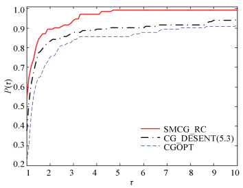
|
Fig.1 Performance profile based on the number of iterations |

|
Fig.2 Performance profile based on the number of function evaluations |
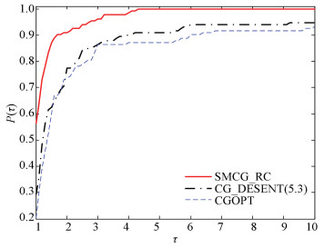
|
Fig.3 Performance profile based on the number of gradient evaluations |
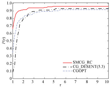
|
Fig.4 Performance profile based on CPU time |
Regarding the number of iterations in Fig. 1, it is worth noting that SMCG_CR is more efficient than CGOPT and CG_DESCENT (5.3), and it smoothly settles about 54% of the test functions with the least number of iterations. The number of test functions it settles are 17% more than CG_DESCENT (5.3) and 31% more than CGOPT. As shown in Fig. 2, it is observed that SMCG_CR is more advanced than CGOPT and CG_DESCENT (5.3) for the number of function evaluations.
Fig. 3 displays the property picture with regard to the number of gradient evaluations. It is easy to observe that the SMCG_CR has the best property, and it smoothly settles about 57% of the test functions with the least number of gradient evaluations. The number of test functions it settles are 28% more than CG_DESCENT (5.3) and 37% more than CGOPT. Fig. 4 displays the performance profile with regard to the CPU time. It can be observed that SMCG_CR is the fastest for about 66% of the test functions, which are 58% test functions faster than CG_DESCENT (5.3) and 31% test functions more than CGOPT. Figs. 1-4 indicate that SMCG_CR outperforms CGOPT and CG_DESCENT (5.3) for the 145 test functions in the CUTEr library.
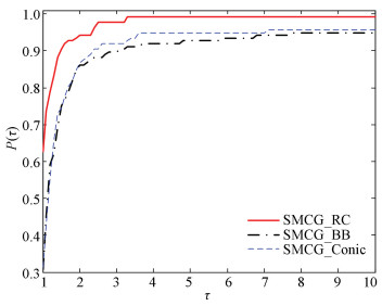
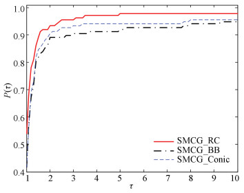
In the second series of the numerical tests, SMCG_CR was compared with SMCG_BB and SMCG_Conic. SMCG_CR successfully solved 142 problems, while SMCG_BB and SMCG_Conic solved 140 and 138 problems, respectively. As shown in Figs. 5-8, SMCG_CR is significantly better than SMCG_BB and SMCG_Conicit for the 145 test functions in the CUTEr library.

|
Fig.5 Performance profile based on the number of iterations |
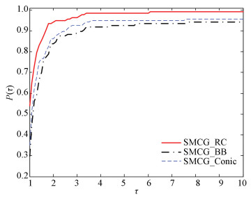
|
Fig.6 Performance profile based on the number of function evaluations |
|
Fig.7 Performance profile based on the number of gradient evaluations |
|
Fig.8 Performance profile based on CPU time |
6 Conclusions
In this paper, a new CG method is presented, which combines subspace technology and a special cubic regularization model. In this method, the sufficient descent condition was satisfied by the search direction. The global convergence of SMCG_CR was built under mild conditions. The numerical experiments showed that SMCG_CR is extraordinarily prospective.
| [1] |
Fletcher R, Reeves C M. Function minimization by conjugate gradients. Computer Journal, 1964, 7(2): 149-154. DOI:10.1093/comjnl/7.2.149 (  0) 0) |
| [2] |
Hestenes M, Stiefel E. Methods of conjugate gradients for solving linear systems. Journal of Research of the National Bureau of Standards, 1952, 49(6): 409-436. DOI:10.6028/jres.049.044 (  0) 0) |
| [3] |
Polyak B T. The conjugate gradient method in extreme problems. USSR Computational Mathematics and Mathematical Physics, 1969, 9(4): 94-112. (  0) 0) |
| [4] |
Dai Y H, Yuan Y X. A nonlinear conjugate gradient method with a strong global convergence property. SIAM Journal on Optimization, 1999, 10(1): 177-182. DOI:10.1137/s1052623497318992 (  0) 0) |
| [5] |
Hager W W, Zhang H C. A new conjugate gradient method with guaranteed descent and an efficient line search. SIAM Journal on Optimization, 2005, 16(1): 170-192. DOI:10.1137/030601880 (  0) 0) |
| [6] |
Hager W W, Zhang H C. A survey of nonlinear conjugate gradient methods. Pacific Journal of Optimization, 2006, 2(1): 35-38. DOI:10.1006/jsco.1995.1040 (  0) 0) |
| [7] |
Rivaie M, Mamat M, Abashar A. A new class of nonlinear conjugate gradient coefficients with exact and inexact line searches. Applied Mathematics and Computation, 2015, 268(1): 1152-1163. DOI:10.1016/j.amc.2015.07.019 (  0) 0) |
| [8] |
Yuan Y X. A modified BFGS algorithm for unconstrained optimization. IMA Journal of Numerical Analysis, 1991, 11(3): 325-332. DOI:10.1093/imanum/11.3.325 (  0) 0) |
| [9] |
Yuan Y X, Stoer J. A review on subspace methods for nonlinear optimization. Proceedings of the International Congress of Mathematics. Seoul, 2014, 807-827. (  0) 0) |
| [10] |
Yuan Y X, Stoer J. A subspace study on conjugate gradient algorithms. ZAMM Journal of Applied Mathematics and Mechanics/Zeitschriftfuer Angewandte Mathematik und Mechanik, 1995, 75(1): 69-77. DOI:10.1002/zamm.19950750118 (  0) 0) |
| [11] |
Li M, Liu H W, Liu Z X. A new subspace minimization conjugate gradient method with non-monotone line search for unconstrained optimization. Numerical Algorithms, 2018, 79: 195-219. DOI:10.1007/s11075-017-0434-6 (  0) 0) |
| [12] |
Cartis C, Gould N I M, Toint P L. Adaptive cubic regularisation methods for unconstrained optimization. Part I: motivation, convergence and numerical results. Mathematical Programming, 2011, 127: 245-295. DOI:10.1007/s10107-009-0286-5 (  0) 0) |
| [13] |
Cartis C, Gould N I M, Toint P L. Adaptive cubic regularisation methods for unconstrained optimization. Part Ⅱ: worst-case function-and derivative-evaluation complexity. Mathematical Programming, 2011, 130: 295-319. DOI:10.1007/s10107-009-0337-y (  0) 0) |
| [14] |
Griewank A. The Modification of Newton*s Method for Unconstrained Optimization by Bounding Cubic Terms. Cambridge: University of Cambridge, 1981.
(  0) 0) |
| [15] |
Hsia Y, Sheu R L, Yuan Y X. Theory and application of p-regularized subproblems for p>2. Optimization Methods and Software, 2017, 32(5): 1059-1077. DOI:10.1080/10556788.2016.1238917 (  0) 0) |
| [16] |
Dai Y H, Yuan J Y, Yuan Y X. Modified two-point stepsize gradient methods for unconstrained optimization problems. Computational Optimization and Applications, 2002, 22: 103-109. DOI:10.1023/A:1014838419611 (  0) 0) |
| [17] |
Moré J J, Garbow B S, Hillstrom K E. Testing unconstrained optimization software. ACM Transactions on Mathematical Software, 1981, 7(1): 17-41. DOI:10.1145/355934.355936 (  0) 0) |
| [18] |
Dai Y H, Kou C X. A Barzilai-Borwein conjugate gradient method. Science China Mathematics, 2016, 59(8): 1511-1524. DOI:10.1007/s11425-016-0279-2 (  0) 0) |
| [19] |
Zhang H C, Hager W W. A nonmonotone line search technique and its application to unconstrained optimization. SIAM Journal on Optimization, 2004, 14(4): 1043-1056. DOI:10.1137/s1052623403428208 (  0) 0) |
| [20] |
Liu Z X, Liu H W. Several efficient gradient methods with approximate optimal stepsizes for large scale unconstrained optimization. Journal of Computation and Applied Mathematics, 2018, 328: 400-413. DOI:10.1016/j.cam.2017.07.035 (  0) 0) |
| [21] |
Gould N I M, Orban D, Toint P L. CUTEr and SifDec: A constrained and unconstrained testing environment, revisited. ACM Transactions on Mathematical Software, 2003, 29(4): 373-394. DOI:10.1145/962437.962439 (  0) 0) |
| [22] |
Dai Y H, Kou C X. A nonlinear conjugate gradient algorithm with an optimal property and an improved Wolfe line search. SIAM Journal on Optimization, 2013, 23(1): 296-320. DOI:10.1137/100813026 (  0) 0) |
| [23] |
Liu H W, Liu Z X. An efficient Barzilai-Borwein conjugate gradient method for unconstrained optimization. Journal of Optimization Theory and Applications, 2019, 180: 876-906. DOI:10.1007/s10957-018-1393-3 (  0) 0) |
| [24] |
Li Y F, Liu Z X, Liu H W. A subspace minimization conjugate gradient method based on conic model for unconstrained optimization. Computational and Applied Mathematics, 2019, 38, Article number: 16(2019). DOI:10.1007/S40314-019-0779-7 (  0) 0) |
| [25] |
Hager W W, Zhang H. The limited memory conjugate gradient method. SIAM Journal on Optimization, 2013, 23(4): 2150-2168. DOI:10.1137/120898097 (  0) 0) |
| [26] |
Nathan C, Autar K, Jai P, et al. Newton-Raphson Method-Graphical Simulation of the Method. http://nm.mathforcollege.com/simulations/mws/03nle/mws_nle_sim_newmet.pdf. [2020-02-12].
(  0) 0) |
| [27] |
Dolan E D, More J J. Benchmarking optimization software with performance profiles. Mathematical Programming, 2002, 91: 201-213. DOI:10.1007/s101070100263 (  0) 0) |
 2021, Vol. 28


