2. School of Mathematical Sciences, Huaibei Normal University, Huaibei 235000, Anhui, China;
3. Department of Mathematics, University of Macau, Macau 999078, China;
4. College of Water Conservancy and Ecological Engineering, Nanchang Institute of Technology, Nanchang 330099, China
It is well-known that most of the problems in biological, physical, electrical science and other scientific areas can be described by partial differential equations (PDEs). Analytical solutions for PDEs are almost inaccessible for relatively complex problems. Numerical approximate solutions of PDEs are an alternative. The traditional mesh-based finite element method[1-3] is stable in early scientific and engineering branches. However, the mesh-generation is a drawback for a large scope of practical demanding problems.
In this study, the emphasis is on the domain-type meshless methods with RBF collocation technique involved. The basic theory of the RBF was derived from the work of Hardy[4], and it was connected with a topology on quadric surface. This type of functions was later applied to simulate PDEs. Edward Kansa in 1990 successfully used a globally supported interpolation, the multiquadric (MQ) RBF, to obtain the approximate solution[5-6]. At present, the Gaussian (GS) RBF is another commonly-used choice in computation[7-10]. It should be pointed out that shape parameters for the MQ and GS should be carefully investigated.
Recently, Biazar and Hosami[11] investigated the shape parameter encountered in RBF approximation. Urleb and Vrankar[12] present a procedure for searching for an optimal shape parameter for the RBF. Besides, the conical type (CT) radial basis function is a parameter-free type[13]. Recently, Reutskiy[14] used the CT RBF to simulate the heat conduction problems. Since the CT RBF is parameter-free, it was compared with MQ and GS in this work.
Because of its good performance, the above-mentioned three radial basis function has been triumphantly applied to solve different PDEs. The numerical solution of three-dimensional (3D) PDEs were considered by Song et al.[15] A finite RBF-based subdomain collocation method was proposed by Chu et al.[16] Numerical and theoretical investigation on the collocation based RBFs have been formulated in Ref. [17]. The RBF was used for solving economic problems[18].
In this work, the above-mentioned three radial basis function, MQ, GS, and CT, were applied to handle PDEs with variable coefficients without iterations. Numerical examples were provided to verify the validity and stability of the three radial basis functions. The parameters in MQ and GS as well as the collocation point numbers were also considered. In Section 1, a description is given for the RBFs. In Section 2, the RBF algorithm is applied to PDEs with variable coefficients. In Section 3, comparative numerical results are illustrated for solving 2D PDEs with variable coefficients. Some conclusions are presented in Section 4.
1 RBFsRBF is a function Φ: Rt→R in case Φ(X)=φ(‖X‖) with φ: [0, ∞)→R and X∈Rt, and t is the space dimensionality.
Interpolation with RBFs takes the following form:
| $ S(X)=\sum\limits_{i=1}^{N} \alpha_{i} \varphi\left(\left\|X-X_{i}\right\|\right) $ | (1) |
The aim is to find the unknown coefficients αi from the system
| $ s\left(X_{i}\right)=f\left(X_{i}\right) $ | (2) |
where X={Xi}i=1N is a given points set in Rt and f(Xi) is a prescribed function. Eq.(1) and (2) have matrix form
| $ \boldsymbol{Q} \alpha=\boldsymbol{f} $ | (3) |
| $ Q_{i j}=\varphi\left\|X_{i}-X_{j}\right\| $ | (4) |
with
| $ \boldsymbol{f}=\left[f\left(X_{1}\right), \ldots, f\left(X_{N}\right)\right]^{\mathrm{T}} $ | (5) |
| $ \boldsymbol{\alpha}=\left[\alpha_{1}, \alpha_{2}, \ldots, \alpha_{N}\right]^{\mathrm{T}} $ | (6) |
where T represents the transpose of vector or matrix. Here, the emphasis is on the three commonly-used RBFs, i.e.,
| $ \varphi(r)=\left(r^{2}+c^{2}\right)^{n / 2} $ | (7) |
where n is an odd integer.
For MQ,
| $ \varphi(r)=\mathrm{e}^{-c^{2} r^{2}} $ | (8) |
For GS,
| $ \varphi(r)=r^{n} $ | (9) |
Consider a linear PDE with variable coefficient operators on a plane domain Ω⊂R2.
| $ L u(X)=f(X), X=(x, y) \in \varOmega $ | (10) |
| $ B u(X)=g(X), X=(x, y) \in \partial \varOmega $ | (11) |
where
| $ L=a \frac{\partial^{2}}{\partial x^{2}}+b \frac{\partial^{2}}{\partial y^{2}}+c \frac{\partial^{2}}{\partial x \partial y}+d \frac{\partial}{\partial x}+e \frac{\partial}{\partial x}+l $ | (12) |
is an operator with a(X), b(X), c(X), d(X), e(X), l(X) as known coefficients. f(X) and g(X) are given functions. B is a linear boundary differential operator.
For the boundary value problem (10)-(11), the basic theory of RBF is given by
| $ \hat{u}\left(X_{i}\right)=\sum\limits_{j=1}^{n} \xi_{j} \varphi\left(r_{i j}\right) $ | (13) |
where φ(·) is a prescribed RBF.
Choose n distinct collocation points {(xj, yj)}j=1n from Ω =(Ω∪∂Ω) with {(xj, yj)}j=1ni in Ω and {(xj, yj)}nj=ni+1 on ∂Ω. To show the numerical solution process, the differentiation of the GS φ(r)=e-c2r2, MQ φ(r)=(r2+c2)n/2 and CT φ(r)=rn are shown in Table 1.
| Table 1 Differentiation of RBFs |
where
| $ r_{j}=\left\|X-X_{j}\right\|=\sqrt{\left(x-x_{j}\right)^{2}+\left(y-y_{j}\right)^{2}} $ | (14) |
Then, substitute Eq.(13) into Eqs.(10)-(11). Eqs.(15) and (16) are obtained:
| $ \sum\limits_{j=1}^{n} \xi_{j} L \varphi\left(r_{i j}\right)=f_{i} $ | (15) |
| $ \sum\limits_{j=1}^{n} \xi_{j} B \varphi\left(r_{i j}\right)=g_{i} $ | (16) |
To be specific, substitute differentiation of the three RBFs into Eqs.(15) and (16), which leads to
| $ \sum\limits_{j=1}^{n} \xi_{j} L \mathrm{e}^{-c^{2} r_{i j}^{2}}=f_{i} $ | (17) |
| $ \sum\limits_{j=1}^{n} \xi_{j} B \mathrm{e}^{-c^{2} r_{i j}^{2}}=g_{i} $ | (18) |
with
| $ \begin{aligned} L \mathrm{e}^{-c^{2} r_{i j}^{2}}=& \mathrm{e}^{-c^{2} r_{i j}^{2}}\left[a\left(X_{i}\right)\left(4 c^{2}\left(x_{i}-x_{j}\right)^{2}-2 c\right)+\right.\\ & b\left(X_{i}\right)\left(4 c^{2}\left(y_{i}-y_{j}\right)^{2}-2 c\right)+\cdots \\ & c\left(X_{i}\right) 4 c^{2}\left(x_{i}-x_{j}\right)\left(y_{i}-y_{j}\right)-\\ & 2 c d\left(X_{i}\right)\left(x_{i}-x_{j}\right)-\\ &\left.2 c e\left(X_{i}\right)\left(y_{i}-y_{j}\right)+l\left(X_{i}\right)\right] \end{aligned} $ | (19) |
for collocating points {(xi, yi)}i=1n. Once {ξj}j=1n are known through solving Eq.(20) and (21), the approximation of u can be obtained. In this work, the numerical algorithm was realized by using MATLAB without iteration.
3 Numerical ExamplesThree benchmark numerical examples were considered in this section. Unless otherwise stated, the solution domain is distributed with evenly interpolation points. The shape parameter c was chosen first, after which the quasi-optimal c was chosen. Numerical results of parameter related MQ and GS were compared with the parameter-free CT for all examples. Besides, n=20 was chosen for MQ and n=11 for CT.
The root mean square error (RMSE) considered is
| $ \operatorname{RMSE}=\sqrt{\frac{1}{T} \sum\limits_{j=1}^{T}\left|\frac{u\left(X_{j}\right)-\hat{u}\left(X_{j}\right)}{u\left(X_{j}\right)}\right|^{2}} $ |
where u(Xj) is the exact solution, û(Xj) is the numerical solution, and T denotes the total interested point number.
3.1 ExamplesCase 1 The equation is given by
| $ \nabla^{2} u+\lambda^{2} u=2 \sin (\mu x) \cos (\mu y)+4 \mu x \cos (\mu x) \cos (\mu y) $ | (20) |
in a square domain. This is the case that a=1, b=1, c=0, d=0, e=0 and l=λ2 and in Eq.(10).
| $ g(x, y)=x^{2} \sin (\mu x) \cos (\mu y) $ | (21) |
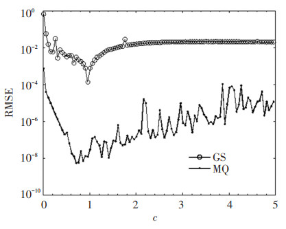
To seek for the quasi-optimal shape parameter c of GS and MQ, a relatively large point number parameter n=20 was initially fixed. The corresponding interior points were generated by MATLAB codes "0.05:1/n: 0.95" with interior point number ni=361 and boundary point on each side was n-1 with boundary point number nt=4n-4=76. Fig. 1 shows the RMSE curves versus the shape parameter c with step interval 0.05. The corresponding condition numbers of the two RBFs are shown in Fig. 2.
|
Fig.1 Influence of the shape parameter c on RMSE for Case 1 |

|
Fig.2 Condition numbers for Case 1 |
Here, the quasi-optimal errors for the GS was obtained by the shape parameter c=0.96 with corresponding RMSE=1.36×10⁻⁴ and the quasi-optimal errors for the MQ was achieved with the shape parameter c=0.71 with corresponding RMSE=5.53×10⁻⁹. This phenomenon reveals that the MQ performed better than the GS for this case. At the same time, it should be noted that the condition numbers for the two RBFs were almost the same for shape parameter c>0.5. This results show that the MQ has better characters than the GS.
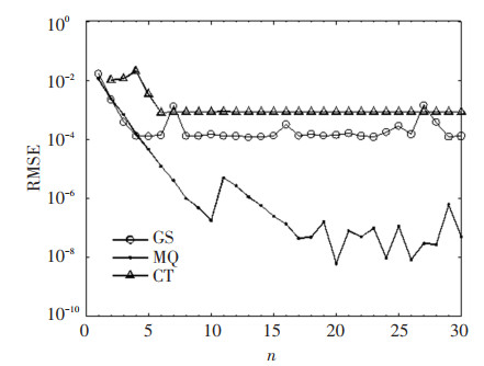
For comparison, convergence curves of the three RBFs with different collocation point number parameters n are shown in Fig. 3. The numerical results of MQ performed better than the GS and CT. But the convergence of CT was more stable than MQ and GS. This phenomenon may be partially attributed to the parameter-free character of the CT case.
|
Fig.3 Convergence curves of the three RBFs with different point number parameter n for Case 1 |
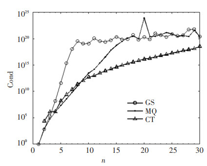
The corresponding condition numbers of the three RBFs are shown in Fig. 4, which shows that the larger condition numbers in Fig. 4 corresponded to the more accurate numerical solutions in Fig. 3. Also, it was found that the larger condition numbers of the MQ and GS corresponded to the better numerical solutions, i.e., the smaller RMSEs. The smaller condition numbers of the CT corresponded to the less accurate numerical solutions, i.e., the bigger RMSEs. Since the results of condition numbers were similar, this issue was ignored in the following two cases.
|
Fig.4 Condition numbers of the three RBFs with different point number parameter n for Case 1 |
Case 2 Consider a heat transfer problem with variable coefficients depicted by Eq.(10). The variable coefficients are
| $ \left\{\begin{array}{l} a=(2 x+y+2)^{2} \\ b=(x+2 y+2)^{2} \\ c=2\left(x-y^{2}\right)^{2} \\ d=10 x+2 y+8 \\ e=2 x+10 y+8 \end{array}\right. $ | (22) |
The Neumann boundary condition was prescribed on y=0 and the rest Dirichlet boundary was chosen properly from the exact solution
| $ u(x, y)=x^{2}+y^{2}-5 x y $ | (23) |
respectively. The corresponding source term is
| $ f(x, y)=-18(x+y)+16 $ | (24) |
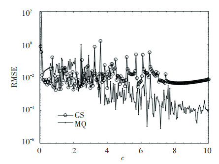
A relatively large point number parameter n=20 was initially fixed, i.e., interior points ni=361 and boundary points nt=76. The curves of RMSE versus the shape parameter c are shown in Fig. 5 with step interval 0.05.
|
Fig.5 RMSE for Case 2 |
Here, the quasi-optimal error RMSE=1.71×10⁻³ for the GS was obtained by the shape parameter c=0.95 and the quasi-optimal RMSE=8.19×10⁻⁶ for the MQ was achieved with the corresponding shape parameter c=7.15. These results reveal that the quasi-optimal error for the MQ is more accurate than the GS one for this case.
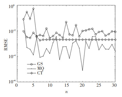
For comparison, convergence curves of the three RBFs with different collocation point number parameters n are shown in Fig. 6, from which it can be found that the MQ performed better than the other two RBFs. However, the convergence of CT was more stable than the MQ and GS. This phenomenon is similar with Case 1.
|
Fig.6 Convergence curves of the three RBFs with different point number parameter n for Case 2 |
Case 3 In this case, the problem
| $ \Delta u-\left(x^{2} y\right) u=f(x, y) $ | (25) |
| $ g(x, y)=\sin \left(y^{2}+x\right)-\cos \left(y-x^{2}\right) $ | (26) |
was considered with the exact solution
| $ u(x, y)=\sin \left(y^{2}+x\right)-\cos \left(y-x^{2}\right) $ | (27) |
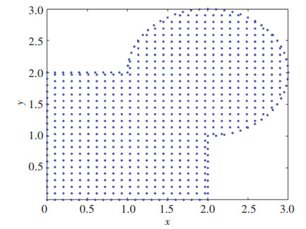
This is the case that a=1, b=1, c=0, d=0, e=0 and l=-x2y in Eq.(10). The calculation domain Ω=Ω1∪Ω2 was formed by (Fig. 7)
| $ \varOmega_{1}=[0, 2] \times[0, 2] $ | (28) |
| $ \begin{aligned} \varOmega_{2}=&\{(x, y) \mid x=\cos \theta+2, y=\sin \theta+2, \\ &\left.-\frac{{\rm{ \mathit{ π} }}}{2} \leqslant \theta \leqslant \frac{{\rm{ \mathit{ π} }}}{2}\right\} \end{aligned} $ | (29) |
|
Fig.7 The irregular domain for Case 3 |
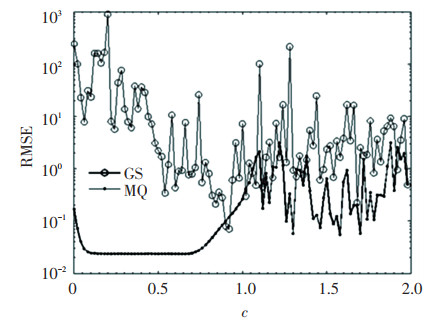
After fixing the 105 points distributed evenly on the boundary domain and 574 interior points spread evenly in the domain, the numerical results are presented with respect to different shape parameters in Fig. 8 for GS and MQ. Here, it is found that RMSE=0.0558 for GS with the quasi-optimal shape parameter c=1.58 and RMSE=0.2357 for the MQ with the corresponding quasi-optimal shape parameter c=0.64, respectively. Both GS and MQ performed not as well as the previous two cases. This may contribute to the irregular computational domain or governing equation. Besides, RMSE=0.0259 was computed for the CT case. Since the variation of collocation point number parameter is difficult to choose, the convergence curves of the three RBFs with different collocation point number parameter are not shown.
|
Fig.8 RMSE for Case 3 |
3.2 Discussions
It can be seen that the three RBFs can be directly applied to solve PDEs with variable coefficients. It is easy to implement and stable with respect to regular or irregular geometry. Regularization techniques are referred to for further investigations[19-20]. Although this paper considers only three cases, the method can be similarly extended to the other cases with minor revision.
4 ConclusionsThe main purpose of this work is to apply the three commonly-used RBFs, i.e., GS, MQ, and CT, for solving PDEs with variable coefficients. Numerical results were provided to show the good performance of the three radial basis functions as numerical tools for a wide range of problems. For some problems the CT one performed not well, but the convergence curves of the errors performed more stable than the other two RBFs. For irregular cases, the three RBFs performed almost the same.
However, a more theoretical and systematic study on the 3D and time-dependent problems is needed to further investigate all RBFs.
| [1] |
Ihlenburg F. Finite Element Analysis of Acoustic Scattering. New York: Springer, 1991. DOI:10.1007/b98828
(  0) 0) |
| [2] |
Wang F Z, Zhang J. New investigations into the MFS for inverse Laplace problems. International Journal of Innovative Computing, Information and Control, 2016, 12(1): 55-66. (  0) 0) |
| [3] |
Zhang J, Wang F Z. Numerical comparisons of two algorithms for Helmholtz-type problems. ICIC Express Letters, Part B: Applications, 2015, 6(3): 859-864. (  0) 0) |
| [4] |
Hardy R L. Multiquadric equations of topography and other irregular surfaces. Journal of Geophysical Research, 1971, 76(8): 1905-1915. DOI:10.1029/JB076i008p01905 (  0) 0) |
| [5] |
Kansa E J. Multiquadrics - A scattered data approximation scheme with applications to computational fluid dynamics I-Surface approximations and partial derivative estimates. Computers & Mathematics with Applications, 1990, 19(8-9): 127-145. DOI:10.1016/0898-1221(90)90270-T (  0) 0) |
| [6] |
Kansa E J. Multiquadrics - A scattered data approximation scheme with applications to computational fluid-dynamics Ⅱ - Solutions to parabolic, hyperbolic and elliptic partial differential equations. Computers & Mathematics with Applications, 1990, 19(8-9): 147-161. DOI:10.1016/0898-1221(90)90271-K (  0) 0) |
| [7] |
McCourt M. Using Gaussian eigenfunctions to solve boundary value problems. Advances in Applied Mathematics and Mechanics, 2013, 5(4): 569-594. DOI:10.1017/S2070073300001399 (  0) 0) |
| [8] |
Zhang Y F, Li C J. A Gaussian RBFs method with regularization for the numerical solution of inverse heat conduction problems. Inverse Problems in Science and Engineering, 2016, 24(9): 1606-1646. DOI:10.1080/17415977.2015.1131825 (  0) 0) |
| [9] |
Zheng K H, Li C C, Wang F Z. Gaussian radial basis function for unsteady groundwater flow. Earth and Environmental Science, 2019, 304(2): 022052. DOI:10.1088/1755-1315/304/2/022052 (  0) 0) |
| [10] |
Karimi N, Kazem S, Ahmadian D, et al. On a generalized Gaussian radial basis function: analysis and applications. Engineering Analysis with Boundary Elements, 2020, 112: 46-57. DOI:10.1016/j.enganabound.2019.11.011 (  0) 0) |
| [11] |
Biazar J, Hosami M. An interval for the shape parameter in radial basis function approximation. Applied Mathematics and Computation, 2017, 315: 131-149. DOI:10.1016/j.amc.2017.07.047 (  0) 0) |
| [12] |
Urleb M, Vrankar L. Searching for an optimal shape parameter for solving a partial differential equation with the radial basis functions method. Engineering Analysis with Boundary Elements, 2018, 92: 225-230. DOI:10.1016/j.enganabound.2017.12.013 (  0) 0) |
| [13] |
Li J C. A radial basis meshless method for solving inverse boundary value problems. Communications in Numerical Methods in Engineering, 2010, 20(1): 51-60. DOI:10.1002/cnm.653 (  0) 0) |
| [14] |
Reutskiy S Y. A meshless radial basis function method for 2D steady-state heat conduction problems in anisotropic and inhomogeneous media. Engineering Analysis with Boundary Elements, 2016, 66: 1-11. DOI:10.1016/j.enganabound.2016.01.013 (  0) 0) |
| [15] |
Song X, Jin Y X, Jiang S X, et al. Meshless global radial point collocation method for three-dimensional partial differential equations. Engineering Analysis with Boundary Elements, 2011, 35(3): 289-297. DOI:10.1016/j.enganabound.2010.10.007 (  0) 0) |
| [16] |
Chu F Y, Wang L H, Zhong Z. Finite subdomain radial basis collocation method. Computational Mechanics, 2014, 54(2): 235-254. DOI:10.1007/s00466-014-0981-9 (  0) 0) |
| [17] |
Larsson E, Shcherbakov V, Heryudono A. A least squares radial basis function partition of unity method for solving PDEs. SIAM Journal on Scientific Computing, 2017, 39: 2538-2563. DOI:10.1137/17M1118087 (  0) 0) |
| [18] |
Rashidinia J, Jamalzadeh S. Collocation method based on modified cubic B-spline for option pricing models. Mathematical Communications, 2017, 22(1): 89-102. (  0) 0) |
| [19] |
Wang F Z, Chen W, Jiang X R. Investigation of regularized techniques for boundary knot method. International Journal for Numerical Methods in Biomedical Engineering, 2010, 26(12): 1868-1877. DOI:10.1002/cnm.1275 (  0) 0) |
| [20] |
Lin J, Chen W, Wang F Z. A new investigation into regularization techniques for the method of fundamental solutions. Mathematics and Computers in Simulation, 2011, 81(6): 1144-1152. DOI:10.1016/j.matcom.2010.10.030 (  0) 0) |
 2021, Vol. 28


