 2022, Vol. 29


Autonomous landing of unmanned aerial vehicle (UAV) is a key part of the autonomous flight process. Data indicates that accidents are most likely to occur at this stage[1]. Vision-based UAV landing has received much attention due to its advantages of strong autonomy. The basic task of such technology is to extract enough image features and use them to solve the attitude and position parameters for UAV's control system[2]. The visual-based landing method can be mainly divided into two categories: 1) cooperative targets deployed on the landing site or runway[3-7], such as artificially placed landing marks; 2) noncooperative targets extracted from images, such as runway edge or horizon[8-10]. The visual landing method based on noncooperative targets does not require manual setting of landing marks, thus has wider applicability[11]. Since most of fixed-wing UAVs must land onto the runway, vision-based navigation method based on the runway has been a hot topic in this field.
Sasa et al.[12] proposed a method using the runway edge and the horizon for position and attitude estimation. The Berkeley team[13] tracked the centerline of runway to determine the yaw angle and horizontal offset of the fixed-wing UAV. Anitha et al.[14] extracted the runway edge and centerline to calculate UAV's position parameters with the known width of runway. Li Hong et al.[15] processed the image of the runway to detect the three feature lines of the runway by Hough transform, then evaluated the offset and yaw angle of the aircraft. Analysis of the above research methods leads to the conclusion that because results of line detection have better accuracy and robustness than that of point, vision-based navigation methods based on the runway mostly estimate the position and attitude parameters with feature lines. However, there is still a problem: the position and attitude information only from runway edgelines is limited without the help of horizon or inertial navigation.
In recent years, the Perspective-N-Point (PNP) problem has been widely used in the fields of photogrammetry, visual measurement, robot control, etc. Scholars have done a lot of research on the accuracy and real-time performance of PNP algorithms. Based on these achievements, this paper selects runway corners as feature to realize six-degree-of-freedom parameter estimation. The main work of this paper consists of two parts: 1) A runway detection algorithm based on long-line feature and gradient projection are proposed, and runway corners are regarded as the intersections of the edgelines in the region of interest, to improve the accuracy and robustness of point detection; 2) Under the premise of known width and length of runway, detected image coordinates are taken as the input of PNP problem, and Orthogonal Iterative (OI) are adopted to improve the accuracy of linear algorithms while avoiding time cost caused by a large number of iterations.
The rest of the paper is organized as follows. Section 1 presents algorithm details for corner extraction. Section 2 introduces the process of OI algorithm. In Section 3, the performance of the above algorithms is validated, and appropriate initial value of iteration is determined for further discussion. Section 4 provides conclusions.
1 Image Processing for LocalizationThe research in this paper has two assumptions: 1) The UAV has been guided to the range of 2 km near the runway, and the direction is aligned with the runway; 2) The forward-looking landing camera is equipped under the UAV. The runway has been clearly visible in the forward-looking images during the research phase. It is trapezoidal from the perspective of UAV, surrounded by obvious sidelines and almost horizontal endlines. Obviously, the extraction of line feature is more stable and accurate than that of point feature at this stage. This section will introduce in detail a runway detection algorithm based on long-line feature and gray-scale feature. Furthermore, corner coordinates are obtained by solving intersections of multiple edgelines. The process can be divided into the following steps: first, locate the region of interest (ROI) using saliency analysis, then detect two sidelines on the binary image based on Hough Transform, finally find the approximate position of upper and lower boundaries through the method of gradient projection.
Fig. 1 is a block diagram of the image process algorithms to extract runway corners as feature points.

|
Fig.1 Block diagram of image process algorithms |
1.1 Region of Interest
The image collected by monocular camera has a huge resolution. If straight lines are directly detected on the original image, the calculation amount is large and it is easily interfered by complex background. Hence, the runway area should be first extracted by ROI segmentation. With reference to the human visual system, when we see a complex scene, we can quickly focus on a specific area of the image. That is region of interest. When UAV landing flight enters the stage of parameter solving, the runway in the forward-looking image has a large contrast with the surrounding environment, such as color and brightness. We try to locate the runway area based on saliency analysis. Saliency analysis method proposed by Hou and Li[16-17] is widely concerned as a global saliency measure based on the spectral residual (SR) of the Fast Fourier Transform (FFT), which favors regions with a unique appearance within the entire image. This method can quickly constructs a saliency map by analyzing the amplitude spectrum of the input image. The biggest advantage is that no prior knowledge is required. Given an image I(x, y), the calculation process includes the following steps.
Step 1: Calculate the amplitude spectrum and phase spectrum according to Eqs. (1) and (2).
| $ A(f)=|F[\boldsymbol{I}(x, y)]| $ | (1) |
| $ P(f)=\varphi(F[\boldsymbol{I}(x, y)]) $ | (2) |
where F[·] denotes the two-dimensional discrete Fourier transform, |·| denotes amplitude, and φ(·) denotes phase. Then the log spectrum L(f) of the image can be obtained as follows:
| $ L(f)=\ln (A(f)) $ | (3) |
Step 2: The spectrum residual R(f) is defined as
| $ R(f)=L(f)-\boldsymbol{h}_{n}(f) \cdot L(f) $ | (4) |
where hn(f) is a n×n matrix defined by
| $ \boldsymbol{h}_{n}(f)=\frac{1}{n^{2}}\left(\begin{array}{cccc} 1 & 1 & \cdots & 1 \\ 1 & 1 & \cdots & 1 \\ \vdots & \vdots & \vdots & \vdots \\ 1 & 1 & \cdots & 1 \end{array}\right) $ | (5) |
Step 3: The saliency map S(x, y) is given as
| $ \boldsymbol{S}(x, y)=g(x) \cdot F^{-1}[\exp (R(f)+P(f))]^{2} $ | (6) |
where g(x) is a Gaussian filter, F-1[·] denotes the inverse Fourier transform.
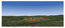
While the saliency map S(x, y) is generated, it is necessary to further use the high saliency characteristics to extract runway target from the image. The sliding window algorithm is classic and most used, which can accurately extract the target. But its low real-time performance is not suitable for landing scenes. A threshold is set to binarize saliency map, which enhances its contrast with background information based on high saliency characteristics of the runway area. Fig. 2 shows the processing effect of the saliency map after binarization. Then, the candidate boxes are extracted by the method of region-labeling[18]. The method overcomes the shortcoming of blind traversal of the sliding window algorithm and reduces the computational complexity.

|
Fig.2 Result of saliency detection |
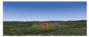
As shown in Fig. 3(a), a large number of candidate boxes are extracted on the binarized saliency map. There are two restrictions which can effectively filter the area containing the runway:

|
Fig.3 Results of candidate box extraction and filtering |
1) Area constraint: Since the UAV has been guided near the runway, target box that contains runway already occupies a large area in the forward view image. Hence, an area threshold can be reasonably set and small candidate boxes are removed.
2) Aspect ratio constraint: Runway usually has predetermined size, for example, the runway in the experimental image is 1000 m long and 60 m wide. During the landing process, the aspect ratio of target box only changes within a certain range. Hence, an aspect ratio threshold can be reasonably set, and the candidate boxes that obviously cannot contain the runway are deleted.
1.2 Runway DetectionWhen the UAV is close to the runway, its edge and plane features are clearly presented in the forward-looking image. The long-line feature is the most obvious. The method of threshold segmentation and line extraction is often adopted in runway detection. As one of the most effective methods to extract straight line, Hough transform has been widely used in runway detection. However, there are still some problems, which affect the accuracy of the detection results.
1) Although the Hough transform can effectively detect two sidelines with long-line feature, due to the influence of noise points and breakpoints, the end points of detected line segments may not be runway corners.
2) The upper edge of the runway is short, and there are many mark lines as interference near the lower edge. If the method of threshold segmentation and line extraction are still used to detect endlines, result may be unreliable.
Therefore, Hough transform was used to realize sideline detection and the gradient feature of runway plane was used to locate endlines, so as to obtain the image coordinates of runway corners based on correct mathematical description of the four edges.
1.2.1 Detection of sidelinesThe long-line feature of sidelines is the most significant feature of runway. Hough transform can provide parameters with high positioning accuracy and good stability. Before line detection, firstly runway edge needs to be separated from the image by threshold segmentation. The key issue is to ensure the segmentation threshold. The paper chooses Otsu segmentation algorithm, which means the maximum separation of target and background in the statistical sense. It is brief and fast. Fig. 4 is the comparison of Otsu algorithm and Niblack algorithm[19], a classic local binary algorithm. It can be seen that the segmentation result of Ostu algorithm eliminates useless details and retains more edge information.

|
Fig.4 Results of threshold segmentation |
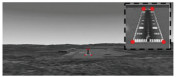
In the Hough transform, the lines through individual non-background points in the image can be represented as sinusoidal curves in the polar coordinate system, where the variable ρ is the distance from the origin to the line along a vector perpendicular to the line and θ is the angle between the x-axis and this vector. If one single line were to pass through these points, then the sinusoidal curves which represents all possible lines through these points would intersect at one single point in the (θ, ρ) plane. The problem of detecting lines is now the problem of finding the Hough peaks in the (θ, ρ) plane. The detection result of sidelines using Hough Transform and corresponding (θ, ρ) plane are illustrated in Fig. 5. Two points of maximum intersection of the sinusoidal curves highlighted in Fig. 5(a) correspond to two runway sidelines in Fig. 5(b).

|
Fig.5 Result of sideline detection using Hough transform |
It is not difficult to see that two longitudinal boundaries in the binary image have obvious length and direction characteristics, which can be used to reduce the huge calculation of traversing every possible θ. Combined with the prior knowledge, the calculation range of θ is reduced to two certain range [10°, 30°] and [-30°, -10°]. As shown in Fig. 6, each sideline corresponds to the Hough peak in one interval.

|
Fig.6 Partial results of right and left edgeline detection |
1.2.2 Detection of endlines
Runway edge on the binarized image is not continuous. There are many breaks. Although Hough transform can locate two sidelines, the determination of the endpoints also requires upper and lower boundary constraints. The runway plane usually has obvious gray-scale differences from the surrounding environment, and there are also obvious mark lines on it. These all determine that the runway zone is an area where gray-scale changes sharply. Since the direction of the UAV has been aligned with the runway, the upper and lower edges of the runway can be approximately replaced with two rows in the image. The gradient magnitude of each pixel in the ROI image was calculated and the gradient magnitude of the row elements were summed. According to the row distribution of gradient magnitude, the beginning and end row of the area were found where pixels with large gradient magnitude are concentrated.
When using the gradient operator to calculate the gradient amplitude, the calculation results of different gradient operators are different. It is expected that a good operator can distinguish the image rows occupied by the runway area from others as much as possible. The paper employs a new operator to process the image. Fig. 7 shows its calculation templates and two other commonly used gradient operators. The processing results of these operators are shown in Fig. 8. The curve obtained by new operator has an obvious rising point in the first half and a sharp drop in the second half, which is similar to the one obtained by Sober operator. In addition, the new operator has a smaller calculation amount than Sober operator.

|
Fig.7 Three gradient operators |

|
Fig.8 Image gradient distribution obtained by three operators |
2 Orthogonal Iteration Algorithm
After using image processing methods to obtain feature point information, it is necessary to further calculate the position and attitude parameters required by the UAV flight control system. What the landing control system needs is the relative position and attitude between the UAV and the runway. In the study, since the camera is installed on the body of the UAV, it is reasonable to assume that the camera reference frame (CRF) and the body-fixed UAV reference frame coincide. The reference frame involved in the position and attitude estimation process is defined as follows:
1) Earth-fixed reference frame (ERF). ERF defined in this paper is built on the runway plane.Select the intersection of the centerline and the starting line of the runway as the origin, the centerline as the x-axis, and the z-axis perpendicular to the ground downwards. Determine the y-axis according to the right-hand rule.
2) Camera reference frame (CRF). CRF was used instead of body-fixed UAV reference frame in this paper. Take the optical center as the origin and the optical axis is the z-axis.
3) Image pixel reference frame (IRF). Take the upper left corner of the image as the origin. The image columns are in accordance with the horizontal coordinates and image rows in accordance with the vertical coordinates.
Therefore, the position and attitude estimation problem of UAV is summarized as follows[20]: finding the conversion relationship between the ERF and the CRF through the three-dimensional coordinates of a set of feature points in the ERF and the corresponding two-dimensional image coordinates. Assuming that the internal parameters of the camera are known, it is a typical PNP problem.
Methods to solve PNP problem can be generally divided into two categories: linear and non-linear algorithms. The accuracy and robustness of linear algorithms are easily affected by image point errors. The non-linear algorithms have the disadvantage of complicated calculation process. The result of position and attitude parameter estimation in UAV landing application must not only be accurate but also stable and robust, and at the same time, it must have high computational efficiency to meet real-time requirements. Orthogonal Iteration (OI) algorithm[21-22] takes the object-space collinearity error as the error function for iterative optimization and has a fast convergence speed. Therefore, this paper adopts an estimation algorithm based on OI.
2.1 Object-Space Collinearity ErrorThe three-dimensional coordinate of feature point expressed in ERF is denoted by Piw(i=1, 2, ···, n), while the corresponding point in CRF is denoted by Qic. For each feature point, there is a rigid transformation relationship:
| $ \boldsymbol{Q}_{i}{ }^{\mathrm{c}}=\boldsymbol{R} \boldsymbol{P}_{i}{ }^{\mathrm{w}}+\boldsymbol{t} $ | (7) |
where R denotes the rotation matrix from the ERF to the CRF and t denotes the translation vector.
Suppose that point vi=[ui vi 1]T is the projection of Piw on the normalized image plane (all points in the plane zc=1 in the CRF). In the idealized pinhole camera model, vi, Qic and the center of projection is collinear. In other words, the collinearity means that the orthogonal projection of Piw on vi should be equal to Qic. Lu et al.[21] and Zhang et al.[22] express the fact by the following equation:
| $ \boldsymbol{R} \boldsymbol{P}_{i}{}^{\mathrm{w}}+\boldsymbol{t}=\boldsymbol{V}_{i}\left(\boldsymbol{R} \boldsymbol{P}_{i}{}^{\mathrm{w}}+\boldsymbol{t}\right) $ | (8) |
where
| $ \boldsymbol{V}_{i}=\left(\boldsymbol{v}_{i} \boldsymbol{v}_{i}{}^{\mathrm{T}}\right)\left(\boldsymbol{v}_{i}{}^{\mathrm{T}} \boldsymbol{v}_{i}\right)^{-1} $ | (9) |
Lu et al.[21] and Zhang et al.[22] refer to Eq. (8) as object-space collinearity equation and further proposes to determine R and t by minimizing the sum of the squared error:
| $ E(\boldsymbol{R}, \boldsymbol{t})=\sum\limits_{i=1}^{n}\left\|\left(\boldsymbol{V}_{i}-\boldsymbol{I}\right)\left(\boldsymbol{R} \boldsymbol{P}_{i}{ }^{\mathrm{w}}+\boldsymbol{t}\right)\right\|^{2} $ | (10) |
The optimal value for t can be expressed by R according to Eq. (11). The OI algorithm rewrittes E(R, t) only with R and computes the rotation matrix by solving the absolute orientation problem during each iteration.
| $ \boldsymbol{t}=\frac{1}{n}\left(\boldsymbol{I}-\frac{1}{n} \sum\limits_{i=1}^{n} \boldsymbol{V}_{i}\right)^{-1} \sum\limits_{i=1}^{n}\left(\boldsymbol{V}_{i}-\boldsymbol{I}\right) \boldsymbol{R} \boldsymbol{P}_{i}{ }^{\mathrm{w}} $ | (11) |
Absolute orientation refers to solving the conversion relationship between the two reference frames based on the three-dimensional coordinates of a set of feature points expressed in two reference frames respectively.
Given corresponding pairs Piw and Qic of three or more noncollinear feature points, the absolute orientation problem is expressed as a constrained optimization problem:
| $ \begin{aligned} &\min \limits_{R, j} \sum\limits_{i=1}^{n}\left\|\boldsymbol{R} \boldsymbol{P}_{i}{ }^{\mathrm{w}}+\boldsymbol{t}-\boldsymbol{Q}_{i}{ }^{\mathrm{c}}\right\|^{2} \\ &\text { s.t. } \quad \boldsymbol{R} \boldsymbol{R}^{\mathrm{T}}=\boldsymbol{I}, \operatorname{det}(\boldsymbol{R})=1 \end{aligned} $ | (12) |
There is a solution method based on the singular value decomposition (SVD)[23]. The basic idea of this method is to convert rigid transformation into pure rotation, thus simplifying the problem.
First, calculate the respective centers of two point sets:
| $ \left\{\begin{array}{l} \mu_{P}=\frac{1}{n} \sum\limits_{i=1}^{n} \boldsymbol{P}_{i}^{\mathrm{w}} \\ \mu_{Q}=\frac{1}{n} \sum\limits_{i=1}^{n} \boldsymbol{Q}_{i}^{\mathrm{c}} \end{array}\right. $ | (13) |
After that, define the following cross-covariance matrix ΣPQ between Qic and Piw:
| $ \Sigma_{P Q}=\frac{1}{n} \sum\limits_{i=1}^{n}\left(\boldsymbol{Q}_{i}^{\mathrm{c}}-\mu_{Q}\right)\left(\boldsymbol{P}_{i}^{\mathrm{w}}-\mu_{P}\right)^{\mathrm{T}} $ | (14) |
Let UDVT be an SVD of ΣPQ, then the optimal rotation matrix can be directly calculated by the following formula:
| $ \boldsymbol{R}=\boldsymbol{U} \boldsymbol{S} \boldsymbol{V}^{\mathrm{T}} $ | (15) |
where
| $ \boldsymbol{S}= \begin{cases}\boldsymbol{I}, & \operatorname{det}\left(\boldsymbol{\Sigma}_{P Q}\right) \geqslant 0 \\ \operatorname{diag}(1, 1, \ldots, 1, -1), & \operatorname{det}\left(\boldsymbol{\Sigma}_{P Q}\right)<0\end{cases} $ | (16) |
The basic idea of the Orthogonal Iterative algorithm is as follows. After obtaining R(k) at the kth iteration, construct the translation vector t(k) and the projection point of Piw on vi, and then solve the absolute orientation problem to obtain R(k+1). Repeat the above steps until the object space collinearity error meets the iteration threshold.
The detailed algorithm steps are summarized as follows:
Step 1: Obtain R(0) by initialization algorithm. Set R(k)=R(0), k=0 and the error threshold as θ;
Step 2: Compute translation vector t(k) according to Eq. (11) and reconstruct the projection point of Piwon vi according to Eq. (8);
Step 3: Compute the sum of the squared error E(R, t). If E(R, t) < θ, stop the iteration and output the results; else, go to the next step.
Step 4: k=k+1, obtain R(k) by solving the absolute orientation problem and return to Step 2.
2.4 Position and Attitude ParameterR and t denote the position and attitude relation between the UAV and runway. From Eq.(7), the relation between Piw and Qic can be expressed in another form:
| $ \boldsymbol{P}_{i}^{\mathrm{w}}=\boldsymbol{R}^{-1} \boldsymbol{Q}_{i}^{\mathrm{c}}-\boldsymbol{R}^{-1} \boldsymbol{t} $ | (17) |
In this paper, the relative position of UAV with respect to runway can be obtained by coordinate of Ow, which represents the origin of the CRF Oc in the ERF.
| $ \boldsymbol{O}^{\mathrm{w}}=-\boldsymbol{R}^{-1} \boldsymbol{t} $ | (18) |
The rotation matrix R is an orthogonal matrix, so R-1=RT. The rotation matrix R contains the attitude change of the CRF, that is, the attitude information of the UAV.
| $ \begin{aligned} \boldsymbol{R}=&\left[\begin{array}{ccc} r_{1} & r_{2} & r_{3} \\ r_{4} & r_{5} & r_{6} \\ r_{7} & r_{8} & r_{9} \end{array}\right]=\\ &\left[\begin{array}{ccc} \mathrm{c} \phi \mathrm{c} \theta & \mathrm{s} \psi \mathrm{s} \theta \mathrm{c} \phi-\mathrm{c} \psi \mathrm{s} \phi & \mathrm{c} \psi \mathrm{s} \theta \mathrm{c} \phi+\mathrm{s} \psi \mathrm{s} \phi \\ \mathrm{s} \phi \mathrm{c} \theta & \mathrm{s} \psi \mathrm{s} \theta \mathrm{s} \phi+\mathrm{c} \psi \mathrm{c} \phi & \mathrm{c} \psi \mathrm{s} \theta \mathrm{s} \phi-\mathrm{s} \psi \mathrm{c} \phi \\ -\mathrm{s} \theta & \mathrm{s} \psi \mathrm{c} \theta & \mathrm{c} \psi \mathrm{c} \theta \end{array}\right] \end{aligned} $ | (19) |
where cx=cos(x), sx=sin(x). ϕ, θ, ψ are the relative rotation angles, referred to as the roll angle, pitch angle, and yaw angle respectively in a flight control system[24]. Hence, attitude parameters can be further solved by Eq. (20):
| $ \left\{\begin{array}{l} \theta=\operatorname{atan}\left(\frac{-r_{7}}{r_{1} \mathrm{c} \phi+r_{4} \mathrm{s} \phi}\right) \\ \phi=\operatorname{atan} \frac{r_{4}}{r_{1}} \\ \psi=\operatorname{atan}\left(\frac{r_{3} \mathrm{s} \phi-r_{6} \mathrm{c} \phi}{r_{5} \mathrm{c} \phi+r_{2} \mathrm{s} \phi}\right) \end{array}\right. $ | (20) |
The proposed algorithms are simulated and analyzed in this section, including algorithms of image processing and algorithms of position and attitude estimation. Matlab 2018 a/b was selected as simulation platform.
3.1 Simulation Results of Image ProcessingSince it is difficult to get images of real landing scenes, the simulative flight software FlightGear[25] was used to generate the videos of UAV autonomous landing and segment the video into images. The resolution of the images was set as 1224×520. 100 images taken by the UAV within 2 km of the runway were selected for the experiment.
3.1.1 ROI detectionIn the algorithm of ROI detection, image scaling factor δ and the threshold τ to obtain a binary saliency map are important parameters which will influence the results of ROI detection and processing time.
Experiment setup: Image resolution is 1224×520, τ is three times the average intensity of the saliency map. Set scaling factor δ to 0.2, 0.4, 0.6, 0.8, and 1, respectively.
The reduction of δ means less image data and less processing time. In addition, Fig. 9 shows that the number of detected candidate boxes decreases as δ decreases, which also means a decrease in processing time.

|
Fig.9 Number of candidate boxes per frame (δ changes) |
Fig. 10 shows the change of ROI in shape corresponding to different δ value. The processing results were further observed and it is found that when δ is small, ROI containing the runway area is irregular in shape and easily contains messy background information, which increases the difficulty of subsequent ROI filter operations. Taking into account processing time and subsequent operations at the same time, this paper chooses δ=0.5. The ROI can be filtered out by searching for the largest candidate box with aspect ratio below 1.5.

|
Fig.10 Two characteristics of ROI (δ changes) |
Experiment setup: Image resolution is 1224×520, δ= 0.5. Calculate the average intensity of the saliency map as E. Starting from E, gradually increase binarization threshold τ.
When τ is small, as shown in Fig. 11, complex background information will interfere with the detection, especially when the runway is far away; when τ is large, as shown in Fig. 12, runway plane details will interfere with the detection, especially when the runway is close.

|
Fig.11 Extraction results of candidate boxes (far, τ changes) |

|
Fig.12 Extraction results of candidate boxes (near, τ changes) |
The results of multiple experiments are counted, and the accuracy of ROI detection under different threshold τ was obtained. Fig. 13 shows that the value of τ is between 3 and 4, with the highest accuracy. Hence, this paper sets τ three times average intensity of the saliency map.

|
Fig.13 Accuracy of ROI detection results (τ changes) |
Experiment setup: Image resolution is 1224×520, δ= 0.5, τ is three times the average intensity of the saliency map.
Table 1 shows the processing results of the proposed method compared with those of the sliding window method. The method proposed in this paper extracted more candidate boxes and took less time. After being filtered by the restrictions of area and aspect ratio, results shown in Table 2 indicate that the algorithms can effectively detect the ROI (from far and near).
| Table 1 Comparison results of candidate box extraction |
| Table 2 ROI detection results of partial frames |


3.1.2 Corner detection
Select 100 images (from far to near) within 2 km from runway to test runway detection algorithm mentioned above and further determine the corner coordinates by the equations of detected lines. Table 3 shows the detection results of partial frames from far and near.
| Table 3 Corner detection results of partial frames |


This paper uses two other methods to compare with the algorithms proposed. One is to adopt only Hough transform for line segment detection, and the other uses Hough transform after mathematical morphology (MM) image processing. The comparison results are shown in Table 4 and the effectiveness of methods is compared from two aspects: success rate and real-time performance.
| Table 4 Comparison results of different detection methods |
It can be seen that the algorithm proposed in this paper can effectively improve the accuracy of corner detection results and has almost no increase in processing time compared with the method only with Hough transform.
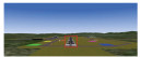
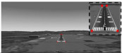
3.2 Simulation Results of Parameter EstimationThe simulation experiments of position and attitude estimation for UAV landing discuss the feasibility and robustness of the presented algorithm. Five points on the runway were selected as shown in Fig. 14 as feature points. Suppose the length of the runway is 1000 m and the width of the runway is 60 m, the coordinates of five feature points in ERF (xw, yw, zw) are demonstrated in Table 5.

|
Fig.14 Five feature points in ERF |
| Table 5 Coordinates of five feature points in ERF |
The estimated errors of landing parameters mainly come from errors of feature point extraction. The errors were compared by adding different levels of random noise to image coordinates of feature points simultaneously. The standard deviation (SD) denotes the level of noise.
3.2.1 Initial valueThe initial value of rotation matrix R affects the accuracy and speed of the OI algorithm in a noisy condition. The experiment compares reproject error of OI algorithm employing different initialization methods. The method Linear_OI obtains initial value of rotation matrix R from camera matrix according to the least-squares solution[26]. Considering that the rotation angles of the UAV change only within a small range in the process of landing[27], the method Constant_OI is to set the initial value of R as a fixed value (such as the matrix, for which ϕ=0, θ=5, ψ=0). EPnP_OI and RPnP_OI methods initialize orientation parameters by EPnP[28] algorithm and RPnP[29] algorithm separately. The comparison results are shown in Table 6.
| Table 6 Error comparison of different initialization algorithms |
It can be seen that estimation results optimized by orthogonal iteration are more accurate than linear algorithm, and the accuracy of iteration results which are obtained by different initialization algorithms is different. The results of Linear_OI, EPnP_OI, and RPnP_OI are more stable and accurate than Constant_OI.
Table 7 compares the processing speeds of different algorithms. From the results, Linear_OI has higher accuracy than linear algorithms, and has the advantage of lower computational complexity within some different initialization methods. Since the position and attitude estimation algorithm used for fixed-wing UAV landing must take both accuracy and real-time performance into account, this paper chooses Linear_OI as the solution method for position and attitude parameters.
| Table 7 Time comparison of different initialization algorithms |
3.2.2 Accuracy and robustness
Linear_OI method was chosen to further study the effect of feature point extraction error on different parameters. Figs. 15-18 shows the estimation errors of six parameters caused by different levels of coordinate errors. The average errors of the entire landing process are given in Table 8.

|
Fig.15 Errors caused by coordinate error with SD=0 |

|
Fig.16 Errors caused by coordinate error with SD=0.01 |

|
Fig.17 Errors caused by coordinate error with SD=0.1 |

|
Fig.18 Errors caused by coordinate error with SD=1 |
It is obvious that estimation errors become greater and greater as SD increases. Results demonstrate that the error of feature point coordinate has a greater impact on the attitude parameters than the position parameters. The figures below show that the coordinate error of the feature point should not exceed SD=0.1.
| Table 8 Error comparison of different parameters |
4 Conclusions
This paper discusses the vision-based relative position and attitude estimation between fixed-wing UAV and runway, which is divided into two parts: corner detection method based on Hough Transform and gradient projection; position and attitude estimation method based on orthogonal iteration. Experiments verified the effectiveness of the corner detection method and show that estimation method has good real-time performance, accuracy, and global convergence when the error of image point coordinate is small. But how to reduce the impact of larger feature point coordinate error is still a problem in practice. References
| [1] |
Marianandam P A, Ghose D. Vision based alignment to Runway during approach for landing of fixed wing UAVs. IFAC Proceedings Volumes, 2014, 47(1): 470-476. DOI:10.3182/20140313-3-IN-3024.00197 (  0) 0) |
| [2] |
Sun Y J, Li Y, Yang H. Runway extraction method based on rotating projection for UAV. Proceedings of the 2016 IEEE 11th Conference on Industrial Electronics and Applications (ICIEA). Piscataway: IEEE, 2016, 421-426. DOI:10.1109/ICIEA.2016.7603621 ( 0) |
| [3] |
Cai M, Sun X X, Xu S, et al. Vision/INS integrated navigation for UAV autonomous landing. Journal of Applied Optics, 2015, 36(3): 343-350. DOI:10.5768/JAO201536.0301002 ( 0) |
| [4] |
Li F, Tan L Z, Tang L. Computer vision assisted UAV landing based on runway lights. Ordnance Industry Automation, 2012, 31(1): 11-13, 36. DOI:10.3969/j.issn.1006-1576.2012.01.004 ( 0) |
| [5] |
Xu G L, Ni L X, Cheng Y H. Key technology of unmanned aerial vehicle's navigation and automatic landing in all weather based on the cooperative object and infrared computer vision. Acta Aeronautica Etastronautica Sinica, 2008, 29(2): 437-442. ( 0) |
| [6] |
Bai L, Chen Q, Teng K J. The computer vision aided auto-landing of UAV. Journal of Projectiles, Rockets, Missiles and Guidance, 2006, 26(2): 320-321, 324. DOI:10.15892/j.cnki.djzdxb.2006.s5.012 ( 0) |
| [7] |
Gui Y, Guo P Y, Zhang H L, et al. Airborne vision-based navigation method for UAV accuracy landing using infrared lamps. Journal of Intelligent & Robotic Systems, 2013, 72(2): 197-218. DOI:10.1007/s10846-013-9819-5 ( 0) |
| [8] |
Zhuang L K, Ding M, Cao Y F. Landing parameters estimation of unmanned aerial vehicle based on horizon and edges of runway. Transducer and Microsystem Technologies, 2010, 29(3): 104-108. DOI:10.13873/j.1000-97872010.03.008 ( 0) |
| [9] |
Zhu F, Liu C, Wu Q X, et al. UAV pose posterior estimation with vision constraint. Robot, 2012, 34(4): 424-431, 439. DOI:10.3724/SP.j.1218.2012.00424 ( 0) |
| [10] |
Zhou L M, Zhong Q, Zhang Y Q, et al. Vision-based landing method using structured line features of runway surface for fixe-wing unmanned aerial vehicles. Journal of National University of Defense Technology, 2016, 38(3): 182-190. DOI:10.11887/j.cn.201603030 ( 0) |
| [11] |
Yang Z G, Li C J. Review on vision-based pose estimation of UAV based on landmark. Proceedings of the 2017 2nd International Conference on Frontiers of Sensors Technologies (ICFST). Piscataway: IEEE, 2017, 453-457. DOI:10.1109/ICFST.2017.8210555 ( 0) |
| [12] |
Sasa S, Gomi H, Ninomiya T, et al. Position and attitude estimation using image processing of runway. Proceedings of the 38th Aerospace Sciences Meeting & Exhibit. Reston, VA: AIAA, 2000. AIAA-2000-0301. DOI: 10.2514/6.2000-301.
( 0) |
| [13] |
Frew E, McGee T, Kim Z W, et al. Vision-based road-following using a small autonomous aircraft. 2004 IEEE Aerospace Conference Proceedings. Piscataway: IEEE, 2004, 3006-3015. DOI:10.1109/AERO.2004.1368106 ( 0) |
| [14] |
Anitha G, Kumar R N G. Vision based autonomous landing of an unmanned aerial vehicle. Procedia Engineering, 2012, 38: 2250-2256. DOI:10.1016/j.proeng.2012.06.271 ( 0) |
| [15] |
Li H, Zhao H Y, Peng J X. Application of cubic spline in navigation for aircraft landing. Journal of Huazhong University of Science and Technology (Nature Science Edition), 2006, 34(6): 22-24. (in Chinese) ( 0) |
| [16] |
Hou X D, Zhang L Q. Saliency detection: a spectral residual approach. Proceedings of the 2007 IEEE Conference on Computer Vision and Pattern Recognition. Piscataway: IEEE, 2007, 15568328. DOI:10.1109/CVPR.2007.383267 ( 0) |
| [17] |
Li J, Duan L Y, Chen X W, et al. Finding the secret of image saliency in the frequency domain. IEEE Transactions on Pattern Analysis and Machine Intelligence, 2015, 37(12): 2428-2440. DOI:10.1109/TPAMI.2015.2424870 ( 0) |
| [18] |
Pan L, Liu Z X. Automatic airport extraction based on improved fuzzy enhancement. Applied Mechanics & Materials, 2011, 130-134: 3421-3424. DOI:10.4028/www.scientific.net/AMM.130-134.3421 ( 0) |
| [19] |
Saxena L P. Niblack's binarization method and its modifications to real-time applications: a review. Artificial Intelligence Review, 2019, 51: 673-709. DOI:10.1007/s10462-017-9574-2 ( 0) |
| [20] |
Maidi M, Didier J Y, Ababsa F, Malik Mallem. A performance study for camera pose estimation using visual marker based tracking. Machine Vision and Applications, 2010, 21: 365-376. DOI:10.1007/s00138-008-0170-y ( 0) |
| [21] |
Lu C P, Hager G D, Mjolsness E. Fast and globally convergent pose estimation from video images. IEEE Transactions on Pattern Analysis and Machine intelligence, 2000, 22(6): 610-622. DOI:10.1109/34.862199 ( 0) |
| [22] |
Zhang Z Y, Zhang J, Zhu D Y. A fast convergent pose estimation algorithm and experiments based on vision images. Acta Aeronautica et Astronautica Sinica, 2007, 28(4): 943-947. ( 0) |
| [23] |
Umeyama S. Least-squares estimation if transformation parameters between two points patterns. IEEE Transactions on Pattern Analysis and Machine Intelligence, 1991, 13(4): 376-380. DOI:10.1109/34.88573 ( 0) |
| [24] |
Zhuang L K, Ding M, Cao Y F. Landing parameters estimation of unmanned aerial vehicle based on horizon and edges of runway. Transducer and Microsystem Technology, 2010, 29(3): 104-108. DOI:10.13873/j.1000-97872010.03.008 ( 0) |
| [25] |
WordPress. Flightgear Flight Simulatior. https://www.flightgear.org.
( 0) |
| [26] |
Hartley R, Zisserman A. Multiple View Geometry in Computer View. Cambridge: Cambridge University Press, 2004.
( 0) |
| [27] |
Fan Y M, Ding M, Cao Y F. Vision algorithms for fixed-wing unmanned aerial vehicle landing system. Science China Technological Sciences, 2017, 60(3): 434-443. DOI:10.1007/s11431-016-0618-3 ( 0) |
| [28] |
Lepetit V, Moreno-Noguer F, Fua P. EPnP: an accurate O(n) solution to the PnP problem. International Journal of Computer Vision, 2009, 81(2): 155-166. DOI:10.1007/s11263-008-0152-6 ( 0) |
| [29] |
Li S Q, Xu C, Xie M. A Robust O(n) Solution to the Perspective-n-Point Problem. IEEE Transactions on Pattern Analysis and Machine Intelligence, 2012, 34(7): 1444-1450. DOI:10.1109/TPAMI.2012.41 ( 0) |