The controller design is usually founded on the mathematical model with the controlled process precisely given in modern control theory. However, the model-based control algorithms often cannot achieve the expected effect in the actual production application due to the unmodeled dynamics and uncertain various factors in the modeling process. In the wake of the progress of science and technology, because of the increasing scale of industrial production and the increasing complexity of the nonlinear system in the actual production process, we cannot get a precise system model in relation to the controlled process. Therefore, we consider designing control methods which are not based on precise mathematical models.
MFC method is a kind of data-driven control (DDC) methods. It only uses the current and past input/output data (IOD) of the controlled process to predict future dynamics. The main MFC methods in the early studies are based on the special linear system structure and the gradient estimation method based on the IOD of the controlled system for general nonlinear systems. Just-in-time modeling is a key step in data-driven control. Just-in-time modeling, also called the instance-based learning[1], on-demand model[2], or delay learning[3], is first proposed in Ref. [4]. Therefore, as an effective control method, scholars have carried out extensive research on MFC method in recent years. Ref. [5] puts forward a model-free adaptive control method (MFAC) in line with the CDL technology regarding a kind of HDNS. The design of the controller only utilizes the IOD of the controlled object to ensure control performance and the convergence towards tracking errors. In allusion to a kind of ordinary discrete-time nonlinear systems which are multi-input and multi-output systems (MIMO), Ref. [6] proposes a data-driven MFAC algorithm based on pseudo-partial derivatives, and the CDL and partial dynamic linearization (PDL) are discussed respectively. Ref. [7] changes the nonlinear time-varying traffic network description into the simplified data model, so that the model-free model has been successfully applied in practice.
MPC is a finite time optimization control method generated from industrial process. MPC includes three fundamental characteristics which are model prediction, rolling optimization, and feedback correction. It is a control strategy that uses the system dynamic model to predict the future system response. Because MPC has the advantages of low requirement on model, easy on-line calculation, and optimization design, in recent years many scholars have combined MPC with model-free method to produce a batch of high-quality control methods. At the beginning of the 21st century, some scholars combined MFAC with MPC and put forward the model-free adaptive predictive control method[8]. However, this method requires the prediction of the pan-model feature vectors at future moments, and the control effect is not ideal due to the imprecise prediction. Therefore, in recent years, it has become a hot topic for some researchers to use the linear model described by pseudo partial derivative matrix (PPDM) to characterize the HDNS, and it has been applied in various domains, for example, food, chemical, industry, aviation, and so on. Ref. [9] presents an MFAC method for a kind of nonlinear systems which are depicted by nonlinear autoregressive moving average model based on Refs. [5] and [6]. Ref. [10] studies the relationship between MFPC and MPC which is grounded on parameter estimation. The noise pollution condition is added into the hypothesis, and the obtained data are optimized to obtain more accurate data. Ref. [11] introduces an MFPC method for nonlinear systems based on polynomial regression expression. The MFPC method based on the linear regression vector of IOD is extended to the polynomial regression vector. Ref. [11] is generalized to MIMO systems in Ref. [12] which realizes its application in wastewater treatment. Ref. [13] proposes a model-free predictive hybrid sensitivity (PHS) H∞ control method based on the IOD to obtain the optimal PHS performance by using the maximum minimization method. Furthermore, it applies the control strategy to the solar power grid system. However, these MFPC algorithms often require a large amount of computation and need to solve complex nonlinear programming problems online, so it is not facile to acquire the explicit analytic solutions. In allusion to a kind of HDNS which have unknown dynamics, an MFSC approach based on the system's IOD and the construction of an adaptive observer to determine the PPDM is proposed in Ref. [14]. But this method has some limitations in system selection and has high-frequency tremor, so the control of some complex industrial processes will become difficult and unsatisfactory.
This paper proposes an MFPC method for a kind of HDNS which are approached by an estimation system. Compared with other nonlinear control algorithms, it not only requires less computation, but also solves the optimization problem, and stables the closed loop system. The remainder of the article is described briefly as follows: in Section 1, the CDL technique is used to establish a data-driven model regarding HDNS. In Section 2, an estimation system is designed and the estimation of the PPDM is given. In Section 3, the prediction model is established, and the appropriate control law is obtained after rolling optimization. Then, the rationality and effectiveness of the method are verified via the simulation results from Section 4. In the end, the summing-up is arranged in Section 5.
1 Question DescriptionConsider the HDNS below, which has an extended external input:
| $ \left\{\begin{array}{l} x_{i}(t+1)=f_{i}\left(x_{1}(t), \cdots, x_{1}\left(t-t_{x_{1 i}}\right), \cdots,\right. \\ \ \ \ \ \left.x_{i+1}(t), \cdots, x_{i+1}\left(t-t_{x_{i+1, i}}\right)\right)(i=1, \cdots n-1) \\ x_{n}(t+1)=f_{n}\left(x_{1}(t), \cdots, x_{1}\left(t-t_{x_{1 n}}\right), \cdots,\right. \\ \ \ \ \ \left.x_{n}(t), \cdots, x_{n}\left(t-t_{x_{n n}}\right), u(t), \cdots, u\left(t-t_{u}\right)\right) \\ y(t)=x_{1}(t) \end{array}\right. $ | (1) |
where xi∈R(i=1, 2, …, n), y∈R, and u∈R are state variables, output, and input of the system, respectively. txi, j and tu denote system orders. The functions fi(·)(i=1, 2, …, n) represent the unidentified smooth functions.
CDL method introduces the concept of PPDM and pseudo-order, and only considers the dynamic relationship between the next moment's output variation and the current moment's input variation. CDL technology can be used to transform the HDNS into a linear time-varying dynamic data model with scalar parameters. In order to adopt the CDL approach, we make the following assumption.
Assumption 1 Partial derivative regarding fi(·)(i=1, 2, …, n-1) in relation to x1(t), …, xi-1(t), xi+1(t), and partial derivative regarding fn(·) in relation to x1(t), …, xn-1(t), u(t) keep continuous. Just for the sake of presentation, let i=1, 2, …, n, if i=n, then, xn+1(t)=u(t).
Theorem 1 Grounded on the above assumption, system (1) can be represented as the following form:
| $ \varDelta \boldsymbol{X}(t+1)=\boldsymbol{H}(t) \boldsymbol{\varLambda}(t) $ | (2) |
where
| $ \varDelta \boldsymbol{X}(t+1)=\left[\varDelta x_{1}(t+1), \cdots, \varDelta x_{n}(t+1)\right]^{\mathrm{T}} $ |
| $ \boldsymbol{\varLambda}(t)=\left[\varDelta x_{1}(t), \cdots, \varDelta x_{n}(t), \varDelta u(t)\right]^{\mathrm{T}} $ |
| $ \varDelta x_{i}(t+1)=x_{i}(t+1)-x_{i}(t) $ |
| $ \varDelta u(t)=u(t)-u(t-1) $ |
| $ \boldsymbol{H}(t)=\left[\begin{array}{ccccc} 0 & \gamma_{12} & \cdots & 0 & 0 \\ \gamma_{21} & 0 & \cdots & 0 & 0 \\ \vdots & \vdots & \ddots & \vdots & \vdots \\ \gamma_{n-1,1} & \gamma_{n-1,2} & \cdots & \gamma_{n-1, n} & 0 \\ \gamma_{n 1} & \gamma_{n 2} & \cdots & 0 & \gamma_{n, n+1} \end{array}\right] $ |
where H(t)∈Rn×(n+1) stands for PPDM, γij represents γij(t).
Proof Let
| $ \begin{aligned} f_{i}^{l}&\left(x_{l}(t-1)\right)=f_{i}\left(x_{1}(t), \cdots, x_{1}\left(t-t_{x_{1 i}}\right), \cdots, \right. \\ &x_{l-1}\left(t-t_{x_{l-1, i}}\right), x_{l}(t-1), x_{l}(t-1), \cdots, \\ &x_{l}\left(t-t_{x_{l i}}\right), \cdots, x_{i+1}(t), \cdots, x_{i+1}(t- \\ &\left.\left.t_{x_{i+1, i}}\right)\right)(l=1, \cdots, i-1, i+1) \end{aligned} $ |
From system (1), the equation is represented as follows:
| $ \varDelta x_{i}(t+1)=\vartheta_{i}+\xi_{i} $ | (3) |
where
| $ \begin{aligned} \vartheta_{i}=&f_{i}(x(t))-\frac{1}{i} f_{i}^{1}\left(x_{1}(t-1)\right)-\cdots-\frac{1}{i} \cdot \\ &f_{i}^{i-1}\left(x_{i-1}(t-1)\right)-\frac{1}{i} f_{i}^{i+1}\left(x_{i+1}(t-1)\right) \end{aligned} $ | (4) |
| $ \begin{aligned} \xi_{i}=&\frac{1}{i} f_{i}^{1}\left(x_{1}(t-1)\right)+\cdots+\frac{1}{i} f_{i}^{i-1}\left(x_{i-1}(t-1)\right)+ \\ &\frac{1}{i} f_{i}^{i+1}\left(x_{i+1}(t-1)\right)-f_{i}(x(t-1)) \end{aligned} $ | (5) |
According to the Lagrange mean value theorem, hereupon
| $ \begin{aligned} \vartheta_{i} &=\frac{1}{i} \frac{\partial f_{i}^{*}}{\partial x_{1}(t)} \varDelta x_{1}(t)+\cdots+\frac{1}{i} \frac{\partial f_{i}^{*}}{\partial x_{i-1}(t)} \varDelta x_{i-1}(t)+\\ &\frac{1}{i} \frac{\partial f_{i}^{*}}{\partial x_{i+1}(t)} \varDelta x_{i+1}(t) \end{aligned} $ | (6) |
where ∂fi*/∂xb(t), (b=1, …, i+1, b≠i) denote the partial derivative regarding fi(·) in relation to xb in [xb(t-1), xb(t)], ∂fn*/∂u(t) represents the partial derivative regarding fn(·) in relation to u in [u(t-1), u(t)].
Similarly, ξi is redescribed as follows:
| $ \begin{aligned} \xi_{i}=&\frac{\partial g_{i 1}^{*}}{\partial x_{1}(t)} \varDelta x_{1}(t)+\frac{\partial g_{i 2}^{*}}{\partial x_{2}(t)} \varDelta x_{2}(t)+\cdots+ \\ &\frac{\partial g_{i, i+1}^{*}}{\partial x_{i+1}(t)} \varDelta x_{i+1}(t)+g_{i, i+1}(x(t)) \end{aligned} $ | (7) |
where
| $ \begin{aligned} g_{i b}&(x(t))=g_{i b}\left(x_{1}(t-1), \cdots, x_{1}\left(t-t_{x_{1 i}}-1\right), \cdots,\right. \\ &x_{b-1}\left(t-t_{x_{b-1, i}}-1\right), x_{b}(t), x_{b}(t-1), \cdots, x_{b}(t- \\ &\left.\left.t_{x_{b i}}-1\right), \cdots, x_{i+1}(t), \cdots, x_{i+1}\left(t-t_{x_{i+1, i}}-1\right)\right) \end{aligned} $ |
∂gib*/∂xb(t) stands for the partial derivative regarding gib(·) in relation to xb in the interval [xb(t-1), xb(t)].
In allusion to every fixed t, the following equation which involve the vector ωi(t) is considered.
| $ g_{i, i+1}=\omega_{i}(t) \varDelta \boldsymbol{\varPsi}(t) $ | (8) |
where ΔΨ(t)=[Δx1(t), …, Δxi-1(t), Δxi+1(t)]T, and Eq. (8) has at least one solution ωi*(t), so there is
| $ \begin{aligned} \xi_{i}=& \beta_{i 1}(t) \varDelta x_{1}(t)+\cdots+\beta_{i, i-1}(t) \varDelta x_{i-1}(t)+\\ & \beta_{i, i+1}(t) \varDelta x_{i+1}(t) \end{aligned} $ | (9) |
where
| $ \beta_{i b}(t)=\frac{\partial g_{i b}^{*}}{\partial x_{b}(t)}+\omega_{i b}(t) $ | (10) |
From Eq. (9), the following equation can be obtained:
In combination with Eqs. (6) and (9), Δxi(t+1) is rewritten as follows:
| $ \begin{aligned} \varDelta x_{i}&(t+1)=\gamma_{i 1} \varDelta x_{1}(t)+\cdots+\gamma_{i, i-1} \varDelta x_{i-1}(t)+ \\ &\gamma_{i, i+1} \varDelta x_{i+1}(t) \end{aligned} $ | (11) |
where
| $ \gamma_{i b}=\frac{1}{i} \frac{\partial f_{i}^{*}}{\partial x_{b}(t)}+\beta_{i b} $ | (12) |
From Eq. (11), Eq. (1) can be represented in another form as Eq. (2).
2 PPDM EstimationThe time-varying parameters of the unknown PPDM are estimated using an approximation in this section. Many algorithms can be chosen, for example, the leakage recursive least squares algorithm, the improved projection algorithm, or the least squares algorithm which has time-varying forgetting factor. Here, an improved projection algorithm is used to estimate PPDM.
Dividing H(t), Λ(t) into blocks, then
| $ \boldsymbol{X}(t+1)=\boldsymbol{X}(t)+\boldsymbol{H}_{1}(t) \boldsymbol{\varLambda}_{1}(t)+\boldsymbol{H}_{2}(t) \Delta u(t) $ | (13) |
where X(t), X(t+1)∈ Rn, H(t)∈ Rn×(n+1), H1(t)∈ Rn×n, H2(t)∈ Rn, Λ1(t)∈ Rn, and Λ(t)∈ Rn+1.
An estimation system is designed as follows:
| $ \hat{\boldsymbol{X}}(t+1)=\hat{\boldsymbol{X}}(t)+\hat{\boldsymbol{H}}_{1}(t) \boldsymbol{\varLambda}_{1}(t)+\hat{\boldsymbol{H}}_{2}(t) \varDelta u(t) $ | (14) |
where
Let
| $ f\left(x, u, \boldsymbol{H}_{1}\right)=\boldsymbol{H}_{1}(t) \boldsymbol{\varLambda}_{1}(t)+\boldsymbol{H}_{2}(t) \varDelta u(t) $ | (15) |
Referring to Ref. [15], the improved projection algorithm is used to estimate PPDM. The pseudo partial derivative estimation criteria is selected as follows:
| $ \begin{aligned} \min &J\left(\hat{\boldsymbol{H}}_{1}(t+1)\right)=\left[\Delta \boldsymbol{X}(t+1)-\bar{f}\left(x, u, \boldsymbol{H}_{1}\right)\right]^{2}+ \\ &\mu_{1}\left(\hat{\boldsymbol{H}}_{1}(t+1)-\hat{\boldsymbol{H}}_{1}(t)\right)^{2} \end{aligned} $ | (16) |
Thereinto, the function
Minimize
| $ \begin{gathered} \hat{\boldsymbol{H}}_{1}(t+1)=\hat{\boldsymbol{H}}_{1}(t)+\frac{1}{\mu_{1}+\left\|\boldsymbol{\varLambda}_{1}(t)\right\|^{2}}\left(\theta _ { 1 } \left(\varDelta \boldsymbol { X } \left(t+\right.\right.\right. \\ \left.\left.1)-\hat{\boldsymbol{H}}_{1}(t) \boldsymbol{\varLambda}_{1}(t)-\hat{\boldsymbol{H}}_{2}(t) \varDelta u(t)\right) \boldsymbol{\varLambda}_{1}^{\mathrm{T}}(t)\right) \end{gathered} $ | (17) |
Similarly,
| $ \begin{gathered} \hat{\boldsymbol{H}}_{2}(t+1)=\hat{\boldsymbol{H}}_{2}(t)+\frac{1}{\mu_{2}+\|\varDelta u(t)\|^{2}}\left(\theta _ { 2 } \left(\Delta \boldsymbol { X } \left(t+\right. \right.\right.\\ \left.\left.1)-\hat{\boldsymbol{H}}_{1}(t) \boldsymbol{\varLambda}_{1}(t)-\hat{\boldsymbol{H}}_{2}(t) \Delta u(t)\right)\right) \Delta u(t) \end{gathered} $ | (18) |
where the constant μ1, μ2>0 are the weight factor.
Let the estimate error about X(t) in the time t be
| $ \boldsymbol{E}(t+1) \leqslant \rho \hat{\boldsymbol{X}}(t+1) $ | (19) |
① According to theorem 2.2 in Ref.[14].
Remark 1: In Eq. (16), a square term with a weighting factor of μ1 is introduced to penalize large parameter errors, which makes the estimation algorithm robust when there are individual abnormal data. It can be seen from Eqs. (17) and (18) that the introduction of μ1, μ2 can avoid the occurrence of zero denominator.
Remark 2: The factors θ1 and θ2 are added to Eqs. (17) and (18) to enhance the generality of the algorithm.
3 MPC 3.1 MPCIn this part, the estimation system (14) is utilized as a prediction model to design a prediction controller.
According to Eq. (13), the system model can be expressed as follows:
| $ \left\{\begin{array}{l} \boldsymbol{X}(t+1)=\boldsymbol{X}(t)+\boldsymbol{H}_{1}(t) \boldsymbol{\varLambda}_{1}(t)+\boldsymbol{H}_{2}(t) \varDelta u(t) \\ \boldsymbol{X}(t+2)=\boldsymbol{X}(t+1)+\boldsymbol{H}_{1}(t+1) \boldsymbol{\varLambda}_{1}(t+1)+ \\ \quad \boldsymbol{H}_{2}(t+1) \varDelta u(t+1) \\ \ \ \vdots \\ \boldsymbol{X}(t+N)=\boldsymbol{X}(t+N-1)+\boldsymbol{H}_{1}(t+N- \\ \quad\quad \text { 1) } \boldsymbol{\varLambda}_{1}(t+N-1)+\boldsymbol{H}_{2}(t+N- \\ \quad \quad \text { 1) } \Delta u(t+N-1) \end{array}\right. $ | (20) |
Unfolding X(t+s)(s=1, 2, …, N-1), which are on the right side of Eq. (20), Eq. (20) can be rewritten as follows:
| $ \boldsymbol{X}_{M}(t)=\boldsymbol{P} \boldsymbol{X}(t)+\boldsymbol{H}_{1 M}(t) \boldsymbol{\varLambda}_{1 M}(t)+\boldsymbol{H}_{2 M}(t) \Delta \boldsymbol{U}(t) $ | (21) |
where
| $ \boldsymbol{X}_{M}(t)=\left[\boldsymbol{X}^{\mathrm{T}}(t+1), \boldsymbol{X}^{\mathrm{T}}(t+2), \cdots, \boldsymbol{X}^{\mathrm{T}}(t+N)\right]^{\mathrm{T}} $ |
| $ \boldsymbol{P}=[\boldsymbol{I}, \boldsymbol{I}, \cdots, \boldsymbol{I}]^{\mathrm{T}} $ |
| $ \varDelta \boldsymbol{U}(t)=[\varDelta u(t), \varDelta u(t+1), \cdots, \varDelta u(t+N-1)]^{\mathrm{T}} $ |
| $ \boldsymbol{\varLambda}_{1 M}(t)=\left[\boldsymbol{\varLambda}_{1}^{\mathrm{T}}(t), \boldsymbol{\varLambda}_{1}^{\mathrm{T}}(t+1), \cdots, \boldsymbol{\varLambda}_{1}^{\mathrm{T}}(t+N-1)\right]^{\mathrm{T}} $ |
| $ \boldsymbol{H}_{i M}(t)=\left[\begin{array}{cccc} \boldsymbol{H}_{i}(t) & 0 & \cdots & 0 \\ \boldsymbol{H}_{i}(t) & \boldsymbol{H}_{i}(t+1) & \cdots & 0 \\ \vdots & \vdots & \ddots & \vdots \\ \boldsymbol{H}_{i}(t) & \boldsymbol{H}_{i}(t+1) & \cdots & \boldsymbol{H}_{i}(t+N-1) \end{array}\right] $ |
where I∈Rn×n is the identity matrix, H1M(t)∈ RnN×nN, H2M(t)∈ RnN×N, P∈ RnN×n, ΔU(t)∈ RN, Λ1M(t)∈RnN, and XM(t)∈ RnN.
At time t, given the prediction of the states about the estimation system (14). Similarly, it can be interpreted as follows:
| $ \hat{\boldsymbol{X}}_{M}(t)=\boldsymbol{P} \hat{\boldsymbol{X}}(t)+\hat{\boldsymbol{H}}_{1 M}(t) \boldsymbol{\varLambda}_{1 M}(t)+\hat{\boldsymbol{H}}_{2 M}(t) \Delta \boldsymbol{U}(t) $ | (22) |
where
| $ \hat{\boldsymbol{H}}_{i M}(t)=\left[\begin{array}{cccc} \hat{\boldsymbol{H}}_{i}(t) & 0 & \cdots & 0 \\ \hat{\boldsymbol{H}}_{i}(t) & \hat{\boldsymbol{H}}_{i}(t+1) & \cdots & 0 \\ \vdots & \vdots & \ddots & \vdots \\ \hat{\boldsymbol{H}}_{i}(t) & \hat{\boldsymbol{H}}_{i}(t+1) & \cdots & \hat{\boldsymbol{H}}_{i}(t+N-1) \end{array}\right] $ |
| $ \hat{\boldsymbol{X}}_{M}(t)=\left[\hat{\boldsymbol{X}}{}^{\mathrm{T}}(t+1), \hat{\boldsymbol{X}}{}^{\mathrm{T}}(t+2), \cdots, \hat{\boldsymbol{X}}{}^{\mathrm{T}}(t+N)\right]^{\mathrm{T}} $ |
where
From Eqs. (21) and (22), the following equation can be deduced:
| $ \boldsymbol{X}_{M}(t)=\hat{\boldsymbol{X}}_{M}(t)+\boldsymbol{E}_{M}(t) $ | (23) |
where
The quadratic function of rolling optimization in finite time domain is used as the performance index:
| $ \min J=\boldsymbol{X}_{M}^{\mathrm{T}}(t) \tilde{\boldsymbol{Q}} \boldsymbol{X}_{M}(t)+\Delta \boldsymbol{U}^{\mathrm{T}}(t) \tilde{\boldsymbol{R}} \Delta \boldsymbol{U}(t) $ | (24) |
thereinto,
Referring to Ref. [16], substitute Eq. (23) to Eq. (24). There is
| $ \begin{gathered} \min J \leqslant\left(2+2 \rho^{2}\right) \hat{\boldsymbol{X}}{}_{M}^{\mathrm{T}}(t) \tilde{\boldsymbol{Q}} \hat{\boldsymbol{X}}_{M}(t)+ \\ \Delta \boldsymbol{U}^{\mathrm{T}}(t) \tilde{\boldsymbol{R}} \Delta \boldsymbol{U}(t) \triangleq \min \hat{J} \end{gathered} $ | (25) |
Eq. (25) means that the minimized optimal solution for
Minimize
| $ \begin{array}{l} \varDelta \boldsymbol{U}(t)=-\left[\left(2+2 \rho^{2}\right) \hat{\boldsymbol{H}}{}_{2 M}^{\mathrm{T}}(t) \tilde{{Q}} \hat{\boldsymbol{H}}_{2 M}(t)+\tilde{R}\right]^{-1} \cdot \\ \ \ \ \ \left(2+2 \rho^{2}\right) \hat{\boldsymbol{H}}{}_{2 M}^{\mathrm{T}}(t) \tilde{\mathrm{Q}}\left(\boldsymbol{P} \hat{\boldsymbol{X}}(t)+\hat{\boldsymbol{H}}_{1 M}(t) \boldsymbol{\varLambda}_{1 M}(t)\right) \end{array} $ | (26) |
Let
| $ u(t)=u(t-1)+\varXi \Delta \boldsymbol{U}(t) $ | (27) |
where
Based on the above analyses, the basic steps of the MFPC algorithm proposed in this paper are as follows:
Step 1: The pseudo-partial derivative estimation matrices
Step 2: Calculate
Step 3: On the basis of the given weight matrices
Step 4: Apply u(t) to system (13) to obtain the system states at the time of t+1.
Step 5: Let t=t+1 and keep up to Step 1.
4 SimulationIn this part, three simulation examples are used to prove the above algorithm.
Example 1:
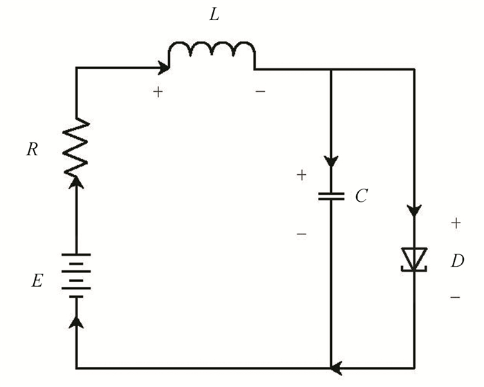
The tunnel diode is a crystal diode whose main current component is the tunnel effect current. It has such characteristics as high speed and high running frequency. Hence, the tunnel diode is widely used in some switching circuits and high frequency oscillation circuits. In this part, the nonlinear model of tunnel diode circuit is taken as an instance to prove the feasibility of the MFPC algorithm.
Considering the tunnel diode circuit which is described in Fig 1, where L, C, R, and D represent inductance, capacitance, resistance, and the tunnel diode, respectively, i and v are the current and voltage passing through the corresponding component. The characteristic of this circuit is iD=h(vD). Define x1=vC, x2=iL, E=u. In this case, L=5, C=2, R=1.5, and h(x1)=17x1-103x12+229x13 are selected. According to Kirchhoff's law of current and voltage, the control system is described as follows:
| $ \left\{\begin{array}{l} \dot{x}_{1}=0.5\left(-17 x_{1}+103 x_{1}^{2}-229 x_{1}^{3}+x_{2}\right) \\ \dot{x}_{2}=0.2\left(-x_{1}-1.5 x_{2}+u\right) \end{array}\right. $ |
|
Fig.1 Tunnel diode circuit |
Let the sample interval be T=0.01 s. The initial states of the system x1(0)=1 and x2(0)=0 are taken. Parameters value are μ1=35, μ2=200, θ1=0.05, θ2=0.01, ρ=0.01,

|
Fig.2 State x1 |

|
Fig.3 State x2 |
|
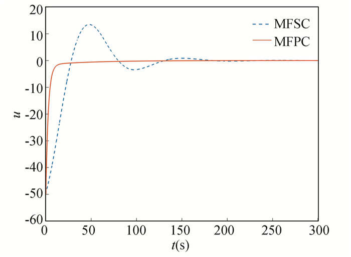
Fig.4 Input u |
|
Fig.5
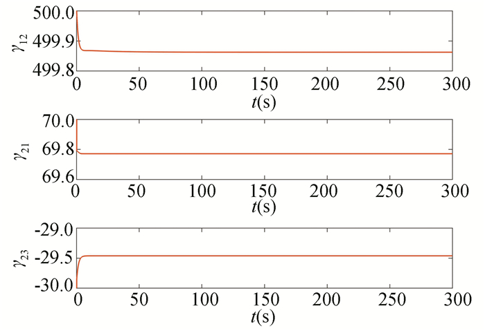
PPDM |
From the simulation results of the tunnel diode circuit, it can come to the conclusions that the MFPC algorithm proposed in this article can warrant that the system states are finally stable for the discrete nonlinear system with unknown system model. The overshoot of the MFPC algorithm is smaller and the system converges faster in comparison with the MFSC algorithm.
Example 2:
The stirred tank system under a standard modeling assumption is taken as an instance to prove the feasibility of the MFPC algorithm. The control system is described as follows:
| $ \left\{\begin{array}{l} \dot{x}_{1}=-2 x_{1}(t)+u(t) \\ \dot{x}_{2}=x_{1}(t)-x_{2}(t)-2 x_{2}^{2}(t) \end{array}\right. $ |
Let the sampling interval be T=0.01 s. Take the initial states of the system x1(0)=1, x2(0)=-10; parameters value are μ1=1, μ2=1, θ1=0.01, θ2=0.1, ρ=0.1,

|
Fig.6 State x1 |
|
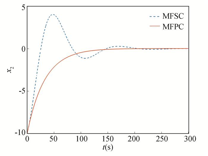
Fig.7 State x2 |
|
Fig.8 Input u |
|
Fig.9
PPDM |
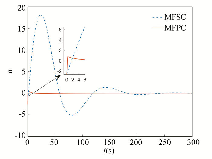
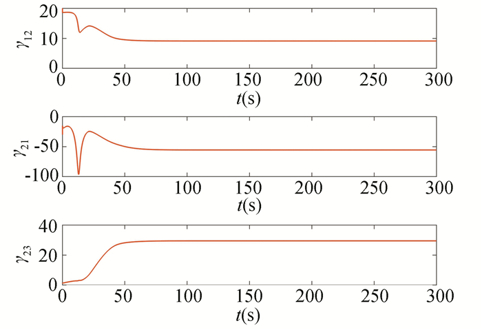
From the above simulation results, it can be seen that both controllers can warrant that the system states are finally stable for the discrete nonlinear system with unknown system model. However, the MFPC can reach stability at about t=100 s, while the MFSC can be stable at about t=200 s. Moreover, compared with the MFSC, the MFPC has less overshoot.
Example 3 (Robust problem):
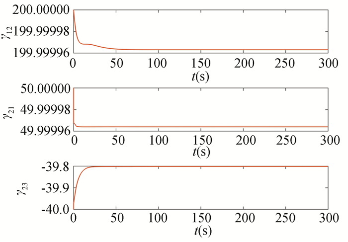
For the system in Example 1, a nonlinear perturbation term is added to the system model:
| $ \left\{\begin{array}{l} \dot{x}_{1}=\frac{1}{2}\left(-17 x_{1}+103 x_{1}^{2}-229 x_{1}^{3}+x_{2}+\sin \left(x_{1}\right)\right) \\ \dot{x}_{2}=\frac{1}{5}\left(-x_{1}-1.5 x_{2}+u\right) \end{array}\right. $ |
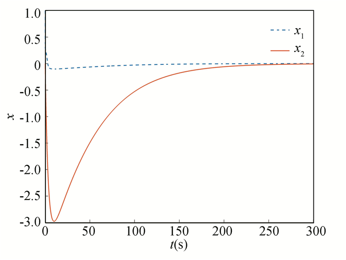
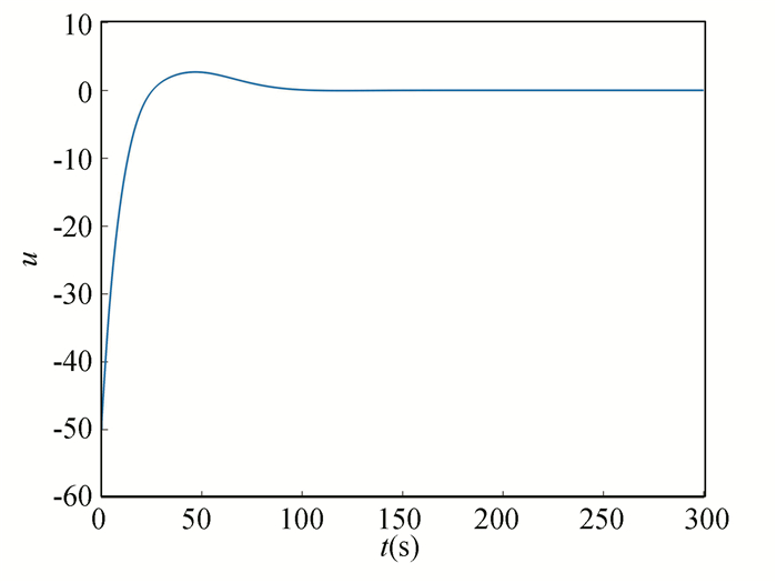
Assuming that the discrete time, initial value, and parameters remain unchanged as in Example 1. The simulation consequences on the basis of the above are given in Figs. 10-12.
|
Fig.10 State x |
|
Fig.11 Input u |
|
Fig.12
PPDM |
It is clear from the above simulation findings, the MFPC suggested in this chapter can still make the system stable after adding the nonlinear disturbance term into the system. Therefore, the MFPC has good robustness.
5 ConclusionsIn this article, an MFPC method is devised for a kind of HDNS whose system models are undefined. The system expressed by pseudo-partial derivative matrix is obtained by compact form dynamic linearization method. The improved projection algorithm is used to design an estimation system to approximate the controlled system. An appropriate predictive controller is designed and the explicit analytical solution of the control is obtained, which finally makes the system stable. The MFPC approach has excellent robustness and stability according to the simulation consequences. Compared with the MFSC method, the MFPC method proposed in this paper has smaller overshoot and faster system convergence. Future works grounded on this article should comprise:
1) expanding the proposed MFPC to MIMO nonlinear systems;
2) the control problems of other special types of nonlinear systems such as fractional order systems with time delay.
| [1] |
Gong C, Liu T L, Tang Y Y. A regularization approach for instance-based superset label learning. IEEE Transactions on Cybernetics, 2017, 48(3): 967-978. DOI:10.1109/TCYB.2017.2669639 (  0) 0) |
| [2] |
Braun M W, Rivera D E, Stenman A. A model-on-demand identification methodology for nonlinear process systems. International Journal of Control, 2001, 74(15): 1708-1717. DOI:10.1080/00207170110089734 (  0) 0) |
| [3] |
Roh S B, Kim Y S, Ahn T C. Lazy learning for nonparametric locally weighted regression. International Journal of Fuzzy Logic and Intelligent Systems, 2020, 20(2): 145-155. DOI:10.5391/IJFIS.2020.20.2.145 (  0) 0) |
| [4] |
Cybenko G. Just-in-time learning and estimation. NATO ASI Series of Computer and Systems Sciences, 1996, 153: 423-434. DOI:10.1007/978-3-662-03295-4_11 (  0) 0) |
| [5] |
Hou Z S, Jin S T. A novel data-driven control approach for a class of discrete-time nonlinear systems. IEEE Transactions on Control Systems Technology, 2011, 19(6): 1549-1558. DOI:10.1109/TCST.2010.2093136 (  0) 0) |
| [6] |
Hou Z S, Jin S T. Data-driven model-free adaptive control for a class of MIMO nonlinear discrete-time systems. IEEE Transactions on Neural Networks, 2011, 22(12): 2173-2188. DOI:10.1109/TNN.2011.2176141 (  0) 0) |
| [7] |
Jin S T, Hou Z S, Chi R H, et al. Model free adaptive predictive control approach for phase splits of urban traffic network. 2016 Chinese Control and Decision Conference. Piscataway: IEEE, 2015, 5750-5754. DOI:10.1109/CCDC.2016.7532027 (  0) 0) |
| [8] |
Cheng Q M, Wang M M, Cheng Y M, et al. Simulation study on model free adaptive control based on grey prediction in ball mill load system. 2010 International Conference on Artificial Intelligence and Computational Intelligence. Piscataway: IEEE, 2010, 422-426. DOI:10.1109/AICI.2010.326 (  0) 0) |
| [9] |
Su C L, Zhang G H, Liu B, et al. Model-free predictive control of nonlinear systems based on linearization of partial format. Proceedings of the 2011 Chinese Control and Decision Conference. Piscataway: IEEE, 2011, 2629-2633. DOI:10.1109/CCDC.2011.5968654 (  0) 0) |
| [10] |
Chaovalit N, Yamamoto S. Model-free predictive control and its relation to parameter-estimation-based predictive control. 2019 SICE International Symposium on Control Systems. Piscataway: IEEE, 2019, 84-89. DOI:10.23919/SICEISCS.2019.8758731 (  0) 0) |
| [11] |
Li H R, Yamamoto S. Polynomial regression-based model-free predictive control for nonlinear systems. Proceedings of the SICE Annual Conference. Piscataway: IEEE, 2016, 20-23. DOI:10.1109/SICE.2016.7749264 (  0) 0) |
| [12] |
Li H R, Yamamoto S. Multi-input multi-output model-free predictive control and its application to wastewater treatment. IEEJ Transactions on Electrical and Electronic Engineering, 2017, 12(5): 753-758. DOI:10.1002/tee.22462 (  0) 0) |
| [13] |
Chen J N, Yang F W, Han Q L. Model-free predictive H∞ control for grid-connected solar power generation systems. IEEE Transactions on Control Systems Technology, 2014, 22(5): 2039-2047. DOI:10.1109/TCST.2013.2292879 (  0) 0) |
| [14] |
Xu D Z, Song X Q, Yan W X, et al. Model-free adaptive command-filtered-backstepping sliding mode control for discrete-time high-order nonlinear systems. Information Sciences, 2019, 485: 141-153. DOI:10.1016/j.ins.2019.02.013 (  0) 0) |
| [15] |
Hou Z S, Jin S T. Model-Free Adaptive Control: Theory and Application. Boca Raton: CRC Press, 2013.
(  0) 0) |
| [16] |
Zhu B, Zheng Z W, Xia X H. Constrained adaptive model-predictive Control for a class of discrete-time linear systems with parametric uncertainties. IEEE Transactions on Automatic Control, 2020, 65(5): 2223-2229. DOI:10.1109/TAC.2019.2939659 (  0) 0) |
 2022, Vol. 29


