In a complex system, there are three common types of dependencies: economic dependence, stochastic dependence and structural dependence[1]. Initially, economic dependence was widely considered in maintenance strategies, while the other two dependencies were rarely mentioned. In these years, Birnbaum importance measure is introduced to effectively consider the system structure, but it does not take the influence of maintenance group into consideration[2-3]. To solve it, a group improvement factor was proposed to formulate a multi-level predictive maintenance[4]. But it did not provide a specific corrective maintenance (CM) rule for component failure. So Ref. [5] proposed an SMRCR rule, but it does not consider component failure accelerates the degradation of other components, i.e., stochastic dependence[2]. Gradually, different maintenance strategies were formulated for the degradation processes and degradation state-rate interactions of components[6-7]. Further, Refs.[8-9] proposed degradation-threshold-shock (DTS) models and stress-strength models (SSM) based on degradation and shock. For the DTS models, the effects of degradation and shocks have been analyzed and different maintenance strategies have been formulated[10-12]. For the SSM, a large number of research results on reliability have appeared based on two different situations. First, when stress and strength are not related, Ref. [13] estimates stress-strength reliability (SSR) and both stress and strength obey gamma distribution; Ref. [14] estimates SSR when both stress and strength follow exponential Weibull distribution. Second, when stress and strength are related, Ref. [15] analyzes a component SSR based on a general two-dimensional distribution; Ref. [16] uses the copula function to describe the dependence between strength and stress and establishes a dependent SSM. However, the above research based on SSM is limited to single-component systems and rarely used for reliability modeling of complex systems.
In response to the above problems, based on Ref.[4], an improved maintenance strategy is proposed. Firstly, system structure is described by component grades and is updated by survival signature. Secondly, considering degradation and shock, SSM and survival signature are introduced to establish a dynamic SSR. Moreover, using group importance measure designed by system dynamic SSR and PM cost, a two-level preventive maintenance (PM) rule is formulated. Finally, a corresponding maintenance strategy model is established, which is optimized by using simulation and genetic algorithm (GA). Further, using a numerical example, this study demonstrates that the developed strategy is useful and effective.
1 System Reliability Modeling 1.1 System DescriptionK(K≥2) types of n components make up a monotonous and coherent system. At initial moment, the system works normally and its components are all new. Let all components status vector be x =(x1, x2, L, xn)∈{0, 1}n. xi=1 indicates the i-th component is in working status. Define ϕ=ϕ(x): {0, 1}n→{0, 1} as system structure function. ϕ(x)=1 indicates the system works normally in view of x. Survival signature is introduced to defined system survival probability, which is rewritten as[17]
| $ \varPhi\left(l_1, l_2, L, l_K\right)=\left[\prod\limits_{k=1}^K\left(\begin{array}{c} m_k \\ l_k \end{array}\right)^{-1}\right] \times \sum\limits_{x \in S_{l_1, l_2, L, l_K}} \phi(x) $ | (1) |
where mk is type k component number, lk is the number of type k components that work normally with k=1, 2, L, K, and Sl1, l2, L, lK is the set of the status vector of components. A 10-component system is used to explain how the survival signature is used. Refer to Appendix for detailed explanation.
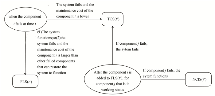
As the change of the component status affects the grades of the system component and ultimately affects the system structure, the four component grades defined in Ref. [5] is used to represent the system structure. The set of the four component grades are critical component set (CCS), temporary critical component set (TCS), failed component set (FLS) and non-critical idle component set (NCIS), respectively. Among the four component grades, the component in CCS will be repaired immediately after failure and the maintenance time is negligible, so it is considered that the components in the grade will not be transferred to other grades. To better exhibit the mutual transformation relationship of the other three component grades, the paper discusses the failure of any component i in the three component grades at time t (Fig. 1). t+ is the time just after time t. Refer to Section 2.1 for detailed description of Fig. 1.
|
Fig.1 Component mutual transformation relationship in TCS, NCIS and FLS |
1.2 Degradation and Shock Modeling of System
Ref.[8] proposes an SSM for components due to degradation and shock. In the SSM, component strength and component stress are two random variables. Component strength refers to the inherent strength for component itself and component stress refers to the external shock, which are denoted by X and Y, respectively. At this point, the dynamic SSR of system or component is defined as the strength greater than the stress, and its mathematical expression is as follows:
| $ R=P(X>Y) $ | (2) |
Eq. (2) reflects the possibility (probability) that the system or component can fully perform their intended function when they work under specified environmental conditions. However, in the field of engineering systems, the strength of some components and systems may deteriorate with time under random stress (such as corrosion, aging, etc.), and the effect of random stress on components and systems may be a cumulative process. So, it is very important to study the multi-system dynamic SSR. The following are the basic assumptions:
1) The initial strength X and random stress Y of the component obey the exponential distribution with parameters α and β, respectively;
2) System components only bear one kind of random stress;
3) Each time a component is subjected to stresses, its strength will degrade by b units and b=0.4. So, when the component is subjected to j cycles of stress Yj=Y, its corresponding strength is Xj=X-jb, and j=1, 2, L.
4) In interval (0, t], the random stress arrival number N(t) acting on the system obeys Poisson distribution with the parameter t/u, u=0.2 is a parameter that number of random stress cycles obey the Poisson distribution.
Based on above assumptions, the cumulative distribution functions (CDF) of related variables are obtained:
| $ F_X\left(x^{\prime}\right)=1-\exp \left(-\alpha x^{\prime}\right), x^{\prime}>0 $ | (3) |
| $ F_Y(y)=1-\exp (-\beta y), y>0 $ | (4) |
| $ \begin{gathered} P(N(t)=j)=\frac{\exp \left(-\frac{t}{u}\right)\left(\frac{t}{u}\right)^j}{j !} \\ t \geqslant 0, j=0, 1, 2, L \end{gathered} $ | (5) |
where x' is an arbitrary real number, y is also an arbitrary real number.
Theorem 1 Let Tsys be the life of the system, then the system dynamic SSR expression at time Tsys=t is
| $ \begin{aligned} & R_{T_{\mathrm{sys}}}(t)=\sum\limits_{l_1=0}^{n_1} L \sum\limits_{l_K=0}^{n_K}\left[\prod\limits_{k=1}^K\left(\begin{array}{c} m_k \\ l_k \end{array}\right)^{-1}\right] \times \\ & \quad \sum\limits_{x \in S_{l_1, L, l_K}} \phi(x) \prod\limits_{k=1}^K\left(\begin{array}{c} m_k \\ l_k \end{array}\right)\left[\frac{\beta_k \gamma}{\alpha_k+\beta_k}\right]^{m_k-l_k}\left[1-\frac{\beta_k \gamma}{\alpha_k+\beta_k}\right]^{l_k} \end{aligned} $ | (6) |
where
Proof Let T' be the life of the component, σj(y) indicates an event that the component has not failed after j cycles of fixed stress Y=y. So the reliability of the component after bearing fixed stress of jth cycle is
| $ \begin{aligned} r_i= & P\left(\sigma_1(y) \cap \sigma_2(y) \cap L \cap \sigma_j(y)\right)= \\ & P(X-j b>Y)=P(X>j b+y)= \\ & \exp (-\alpha(y+j b)) \end{aligned} $ | (7) |
When Y is unknown, the reliability of the component after bearing random stress of jth cycle is
| $ \begin{aligned} R_j= & \int_0^{\infty} \exp (-\alpha(y+j b)) f_Y(y) \mathrm{d} y=\frac{\beta}{\alpha+\beta} \exp (- \\ & j \alpha b) \end{aligned} $ | (8) |
Combining Eq. (5), component SSR at time T'=t can be obtained, namely,
| $ \begin{aligned} & R_{T^{\prime}}(t)=\sum\limits_{j=0}^{\infty} R_j P(N(t)=j)= \\ & \sum\limits_{j=0}^{\infty} \frac{\beta}{\alpha+\beta} \exp (-j \alpha b) \frac{\exp \left(-\frac{t}{u}\right)\left(\frac{t}{u}\right)^j}{j !}= \\ & \frac{\beta}{\alpha+\beta} \exp \left(-\frac{(1-\exp (-\alpha b)) t}{u}\right), t \geqslant 0 \end{aligned} $ | (9) |
Using Eq. (9) can calculate the SSR of the type k components at time T'=t, namely,
| $ R_{T^{\prime}}^k(t)=\frac{\beta_k}{\alpha_k+\beta_k} \exp \left(-\frac{\left(1-\exp \left(-\alpha_k b\right)\right) t}{u}\right) $ | (10) |
In a monotonous and coherent system, survival signature can be used to describe the working status of the system, and the system structure can be separated from the probability model that describes component random failure. So, survival signature is widely used to calculate the system reliability, i.e.,
| $ \begin{aligned} & R_{T_{\mathrm{sys}}}(t)=\sum\limits_{l_1=0}^{n_1} L \sum\limits_{l_K=0}^{n_K} \varPhi\left(l_1, L, l_K\right) P\left(\bigcap\limits_{k=1}^K\left(C_t^k=l_k\right)\right)= \\ & \quad \sum\limits_{l_1=0}^{n_1} L \sum\limits_{l_K=0}^{n_K}\left[\prod\limits_{k=1}^K\left(\begin{array}{c} m_k \\ l_k \end{array}\right)^{-1}\right] \times \sum\limits_{x \in S_{l_1, L, l_K}} \phi(x) \prod\limits_{k=1}^K\left(\begin{array}{c} m_k \\ l_k \end{array}\right) . \\ & \quad\left[1-R_{T^{\prime}}^k(t)\right]^{m_k-l_k}\left[R_{T^{\prime}}^k(t)\right]^{l_k} \end{aligned} $ | (11) |
Based on Eq. (1) and Eqs. (10)-(11), the system dynamics SSR at time Tsys=t can be obtained, namely,
| $ \begin{aligned} & R_{T_{\mathrm{sys}}}(t)=\sum\limits_{l_1=0}^{n_1} \cdots \sum\limits_{l_K=0}^{n_K}\left[\prod\limits_{k=1}^K\left(\begin{array}{c} m_k \\ l_k \end{array}\right)^{-1}\right] \times \\ & \sum\limits_{x \in S_{l_1, L, l_K}} \phi(x) \prod\limits_{k=1}^K\left(\begin{array}{c} m_k \\ l_k \end{array}\right) \cdot \\ & {\left[\frac{\beta_k}{\alpha_k+\beta_k} \exp \left(-\frac{\left(1-\exp \left(-\alpha_k b\right)\right) t}{u}\right)\right]^{m_k-l_k} \cdot }\\ & {\left[1-\frac{\beta_k}{\alpha_k+\beta_k} \exp \left(-\frac{\left(1-\exp \left(-\alpha_k b\right)\right) t}{u}\right)\right]^{l_k}} \end{aligned} $ | (12) |
The proof is completed.
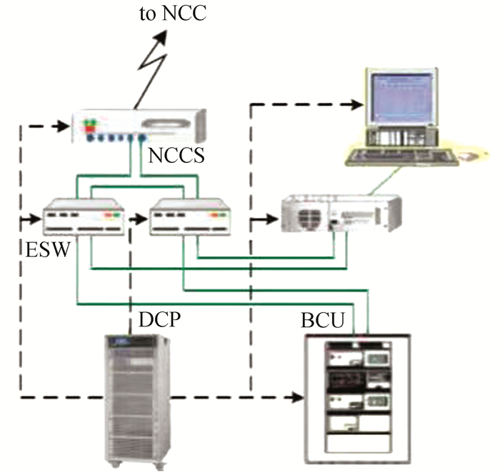
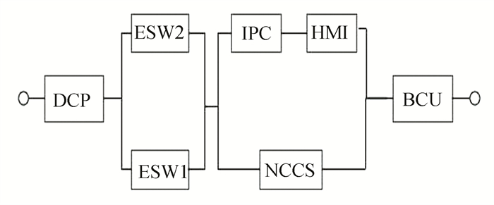
The following takes the substation system[18] as an example to analyze the system dynamic SSR by comparing it with the system reliability that only considers the internal degradation of the components. Their topology and configuration are given, as shown in Fig. 2 and Fig. 3. The substation system relevant data are listed in Table 1.
|
Fig.2 Topology of a substation system |
|
Fig.3 Reliability block diagram of substation system |
| Table 1 Substation system parameter data |
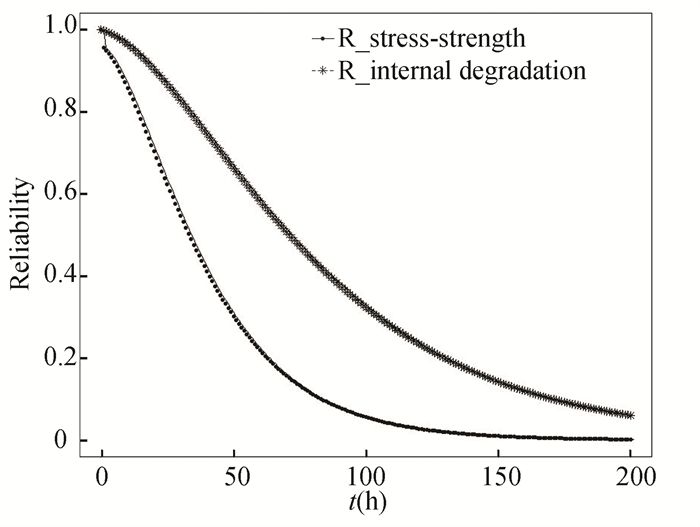
The calculating result of the two system reliabilities are shown in Fig. 4. The results indicate both system reliabilities decrease with time, but the system dynamic SSR decreases faster, because for the system dynamic SSR, it takes into account internal degradation and external shock. Obviously, the results are realistic.
|
Fig.4 Comparison of system reliability |
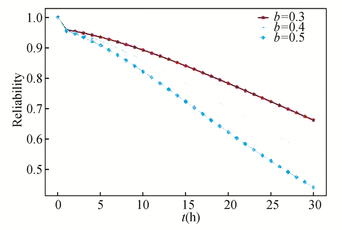
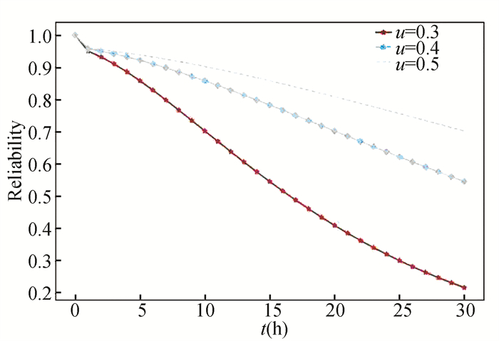
Fig. 5 and Fig. 6 show sensitivity analysis result with parameters b and u, respectively. Fig. 5 shows when b increases, the system dynamic SSR also increases. Because the larger the value of b, the larger the degree of strength degradation becomes, and ultimately the smaller the system survival probability becomes. Fig. 6 shows when u increases, the system dynamic SSR decreases. Because when u increases, the arrival frequency of external shock is reduced, which makes the number of the component subjected to external shock reduce.
|
Fig.5 Sensitivity analysis of b |
|
Fig.6 Sensitivity analysis of u |
The analysis indicates that it is meaningful to establish the system dynamic SSR. The following applies the dynamic SSR to system maintenance strategy. To simplify the subsequent related model, the following assumptions are made:
1) At a certain moment, only one component fails;
2) Preventive maintenance and corrective replacement are the replacement of an original component with a brand new one, while minimal repair is the repair of the original faulty component;
3) Maintenance durations of system components are 0;
4) Necessary maintenance resources are always available.
2 Maintenance StrategyInternal degradation and external shock will cause system component failure, which affects the system structure. So, an SMRCR is formulated. In addition, to reduce maintenance cost, a preventive maintenance rule is formulated considering the group importance measure.
2.1 System Structure UpdatingLet Stru (t0) be system structure at time t0. The dependency relationship of system structure and component grade sets is given at time t0, namely,
| $ \begin{aligned} {\bf{Stru}}(t) & =[\operatorname{CCS}(t), \operatorname{TCS}(t), \operatorname{NCIS}(t), \\ & \operatorname{FLS}(t)] \end{aligned} $ | (13) |
Based on Eq. (13), a component failure leads to component grade updating, which ultimately leads to system structure updating. Next, the system structure updating process with component failure is given based on Fig. 1.
Firstly, a status-survival matrix is defined based on the survival signature at time t0, i.e.,
| $ \operatorname{Mat}\left(i, t_0\right)=\left(S_{l_1, l_2, L, l_K} \varPhi\left(l_1, L, l_K\right)\right)_{x=\left(x_1, L, 0_i, L, x_n\right)} $ | (14) |
Mat(i, t0) reflects the status vector when component i fails at time t0. Then, a function is defined as follows:
| $ \operatorname{summ}\left(i, t_0\right)=\sum\limits_{x=\left(x_1, L, 0_i, L, x_n\right)} \varPhi\left(l_1, l_2, L, l_K\right) $ | (15) |
Eq. (15) is calculated by the last column of the row corresponding to xi=0 in the status-survival matrix at time t0, and it reflects and quantifies the impact degree of component i failure on the system at time t0. If summ(i, t0)=0, it means component i failure causes system failure. When component w fails at time tfw, let tfw- and tfw+ be the time before and after tfw, respectively.
(ⅰ) If the component w is in CCS(tfw-), Stru(tfw-)=Stru(tfw+) is obtained.
(ⅱ) If the component w is not in CCS(tfw-) Mat(w, tfw) and summ(w, tfw) are obtained based on Eq. (1) and Eqs. (14)-(15). The following step is to renew component grades after component w fails based on Fig. 1 as follows:
Case A If summ(w, tfw)≠0, component w failure does not cause system failure, so the component w is removed from the original component grade set and stored in FLS(tfw+). At this time, if the working component q is in CCS(tfw-), the component grade of q remains unchanged, and summ(q, tfw) is obtained. If summ(q, tfw)=0, q is removed from the original component grade set and stored in TCS(tfw+). Otherwise, q is stored in NCIS(tfw+).
Case B If summ(w, tfw)=0, the component w is temporary critical component at time tfw-. Let Citfw be CM cost of component i at time tfwand be defined as follows:
| $ C_i^{t f_w}=c_{m, i} I_{\left\{n_0[i]<l\right\}}+c_{c, i} I_{\left\{n_0[i]=l\right\}} $ | (16) |
where n0[i] is the number of consecutive minimal repair of component i. Let SE(tfw) be a set of failed components, and when any component in SE(tfw) is restored to working status, the failed system can be restored to working status at time tfw.
For any component g in SE(tfw) and g≠w, Chtfw=min(Cwtfw, Cgtfw) can be obtained based on Eq. (16) and component h needs to be executed by CM immediately.
1) If h=w, system component grades are constant, i.e., Stru(tfw-)=Stru(tfw+).
2) If h=g, w is removed from the original component grade set and stored in FLS(tfw+), and g is removed from FLS(tfw-) and stored in TCS(tfw+). At this time, Mat(w, tfw+) is obtained. For the working component d, if d is in CCS(tfw-), component d grade remains unchanged. Otherwise, summ(d, tfw+) is calculated based on Mat(w, tfw+). If summ(d, tfw+)=0, component d is stored in TCS(tfw+). Otherwise, it is stored in NCIS(tfw+).
Finally, the system structure is updated based on (ⅰ) and (ⅱ) at time tfw+ as follows:
| $ \begin{aligned} \operatorname{Stru}\left(t f_w^{+}\right)= & {\left[\operatorname{CCS}\left(t f_w^{+}\right), \operatorname{TCS}\left(t f_w^{+}, \right) \operatorname{NCIS}\left(t f_w^{+}\right)\right.} \\ & \left.\operatorname{FLS}\left(t f_w^{+}\right)\right] \end{aligned} $ | (17) |
Minimal repair (MR) reduces cost and corrective replacement (CR) improves system reliability. Considering their advantages, this subsection proposes an SMRCR rule by updating system structure. When component w fails at time tfw, three cases are discussed:
1) If w is in CCS(tfw-), it needs to be repaired immediately. If n0[w] < l, MR is selected. Otherwise, CR is selected.
2) If wis in TCS(tfw-), for q in SE(tfw) and q≠w, Chtfw=min(Cwtfw, Cqtfw) is calculated by using Eq. (16). Now, component h is repaired immediately. If n0[h] < l, h is executed MR. If n0[h]=l, h is executed CR.
3) If w is in NCIS(tfw-), w keeps fail.
2.3 Group Importance Measure Based on System Dynamics SSRIn the existing PM rules, it is rare to take into account the importance measure of several components together. So group importance measure is designed as follows:
| $ I M^{G_z}\left(T_r\right)=\frac{R_{T_{\mathrm{sys}}}^{G_z}\left(T_r\right)}{C^{G_z}} $ | (18) |
where
1) RTsysGz(Tr) is system dynamics SSR after all components in Gz are preventively replaced at time Tr, Gz is the z-th group of components and Tsys is system life. It should be noted that when the type k components in group Gz are preventively replaced, SSR of all corresponding components at this time is 1, i.e.,
| $ R_{T^{\prime}}^k\left(T_r\right)=1 $ | (19) |
For the type k components outside group Gz, their SSR are obtained based on Eq. (10), i.e.,
| $ R_{T^{\prime}}^k\left(T_r\right)=\frac{\beta_k}{\alpha_k+\beta_k} \exp \left(-\frac{\left(1-\exp \left(-\alpha_k b\right)\right) T_r}{\lambda}\right) $ | (20) |
where T' is component life. Finally, substituting Eq. (19) and Eq. (20) into Eq. (11), RTsysGz(Tr) is obtained.
2) CGz is PM cost for Gz.
| $ \begin{aligned} & C^{G_z}=\sum\limits_{i \in G_z}\left(c_{p, i}+c_s\right)-c_s\left(\left|G_z\right|-1\right)- \\ & c_{\mathrm{psd}}\left(\sum\limits_{i \in G_z} I_{\left\{i \in \operatorname{CCS}\left(T_r\right) \cup \operatorname{TCS}\left(T_r\right)\right\}}-I_{\left\{G_z \text { is a critical group }\right\}}\right) \end{aligned} $ | (21) |
where I{ } is an indicator function. I{ }=1 if { } is true and I{ }=0 if not. Gz is defined as a critical group when the failures of one or more components in Gz cause system failure. cs(|Gz|-1) is set-up cost saving because of positive economic dependence (PED) between components.
| $ c_{\mathrm{psd}}\left(\sum\limits_{i \in G_z} I_{\left\{i \in \operatorname{CCS}\left(T_r\right) \cup \operatorname{TCS}\left(T_r\right)\right\}}-I_{\left\{G_z \text { is a critical group }\right\}}\right) $ |
is planned shutdown cost saving owing to Gz.
2.4 Two-Level PM ruleA two-level PM rule is executed at time Tr=rT, r=1, 2, L, which considers group importance measure. The two-level includes system level and component level.
2.4.1 System levelSystem dynamics SSR, i.e., RTsys(Tr-) is firstly calculated by Eq. (6), then compared with reliability threshold R0(0 < R0≤1). If RTsys(Tr-) < R0, the next step is to seek an optimal component group to be replaced, which occurs at the component level.
2.4.2 Component levelUnder certain conditions, comparison of their group importance measures can find the optimal component group to be replaced. At time Tr, if a components are working, possible group number is 2a-1. Group Gz is acceptable if RTsysGz(Tr)>R0. By comparing all acceptable groups, an optimal group Gz* is found as the one with the highest value of group importance measure. The specific expression is as follows:
| $ I M^{G_z^*}\left(T_r\right)=\max\limits_{z=1, 2, L, 2^a-1}\left\{I M^{G_z}\left(T_r\right) \mid R_{T_{\mathrm{sys}}}^{G_z}\left(T_r\right)>R_0\right\} $ | (22) |
Based on the proposed maintenance strategy, cost-rate is defined as follows[3]:
| $ \begin{aligned} & \operatorname{CR}\left(T, R_0\right)=\lim _{M \rightarrow \infty} \operatorname{CR}\left(M \mid T, R_0\right)= \\ & \lim _{M \rightarrow \infty} \frac{\sum\limits_{r=1}^M\left(C_{T_r}^{\mathrm{insp}}+C_{T_r}^{\mathrm{prev}}+C_{T_r}^{\text {corr }}+C_{\left(T_{r-1}, T_r\right)}^{\mathrm{corr}}\right)}{M T} \simeq \\ & \frac{\sum\limits_{r=1}^{\tilde{M}}\left(C_{T_r}^{\mathrm{insp}}+C_{T_r}^{\text {prev }}+C_{T_r}^{\text {corr }}+C_{\left(T_{r-1}, T_r\right)}^{\mathrm{corr}}\right)}{\tilde{M} T} \end{aligned} $ | (23) |
where CR(M|T, R0|) is cost-rate within M first planned maintenance periods.
CTrinsp is only the inspection operations cost of surviving components at time Tr. It is calculated as follows:
| $ C_{T_r}^{\mathrm{insp}}=c_{\text {insp }}\left(n-\sum\limits_{i \in \varOmega \backslash G_z^*} I_{\left\{i \in \operatorname{FLS}\left(T_r\right)\right\}}\right) $ | (24) |
where Ω\Gz* is the set of components outside the group Gz*.
CTrprev is total PM cost at time Tr, which contains preventive replacement cost for every component in Gz*, set-up cost and the planned shutdown cost. Owing to the PED of components in group Gz*, set-up cost is distributed only once when maintenance is executed at time Tr. CTrprev is calculated by
| $ \begin{aligned} C_{T_r}^{\text {prev }} & =\sum\limits_{i \in G_z^*}\left(c_{p, i}+c_s\right)-c_s\left(\left|G_z^*\right|-1\right)- \\ & c_{\mathrm{psd}}\left(\sum\limits_{i \in G_z^*} I_{\left\{i \in \operatorname{CCS}\left(T_r^{-}\right) \cup \operatorname{TCS}\left(T_r^{-}\right)\right\}}-I_{\left\{G_z^* \text { is a critical group }\right\}}\right) \end{aligned} $ | (25) |
C(Tr-1corr, Tr) is total CM cost in the r-th maintenance cycle, which contains CR cost, MR cost, set-up cost and unplanned shutdown cost. If component w fails at time tfw with Tr-1 < tfw < Tr, C(Tr-1corr, Tr) is calculated as follows:
| $ \begin{array}{r} C_{\left(T_{r-1}, T_r\right)}^{\mathrm{corr}}=\sum\limits_{w \in \mathrm{FLS}\left(tf_w\right)}\left(c_{m, w} I_{\left\{n_0[w]<l\right\}}+c_{c, w} I_{\left\{n_0[w]=l\right\}}+\right. \\ \left.c_s\right)+\sum\limits_{w \in \operatorname{FLS}\left(t f_w\right)} c_{\text {usd }} I_{\left\{w \in \operatorname{CCS}\left(t f_w^{-}\right) \cup \operatorname{TCS}\left(t f_w^{-}\right)\right\}} \end{array} $ | (26) |
CTrcorr is CM cost at time Tr, and contains CR or MR cost. CTrcorr is calculated as follows:
| $ C_{T_r}^{\text {corr }}=\sum\limits_{w \in \varOmega \backslash G_z^*}\left(c_{m, w} I_{\left\{n_0[w]<l\right\}}+c_{c, w} I_{\left\{n_0[w]=l\right\}}\right) I_{\left\{w \in \operatorname{FLS}\left(T_r\right)\right\}} $ | (27) |
Consequently, from Eqs. (23)-(27), CR(T, R0) is calculated. Finally, by minimising cost-rate, the optimal values (T, R0) is found, i.e.,
| $ \operatorname{CR}\left(T^*, R_0^*\right)=\min\limits_{T>0, R_0 \in(0, 1]}\left\{\operatorname{CR}\left(T, R_0\right)\right\} $ | (28) |
Based on Eqs.(23)-(27), simple analytical method cannot evaluate the cost-rate. So, GA is considered in Ref. [3], which is done only with
| $ \begin{aligned} \Delta \mathrm{CR}=&\max _{j=\tilde{M}-\varepsilon, L, \tilde{M}} \mathrm{CR}\left(j \mid T, R_0\right)- \\ & \min _{j=\tilde{M}-\varepsilon, L, \tilde{M}} \operatorname{CR}\left(j \mid T, R_0\right) \leqslant \triangle \mathrm{CR}^0 \end{aligned} $ | (29) |
where △CR0=0.01 is convergence tolerance. The integer
This section takes the substation system of Fig. 2 as an example to optimize and evaluate the proposed strategy. Finally, the paper analyses parameter sensitivity. The relevant cost parameters are listed in Table 2.
| Table 2 Substation system relevant cost parameters |
3.1 Optimization of Maintenance Strategy Model
The maintenance strategy model in Section 2.5 is very complex, so the strategy is optimized by simulation analysis and GA[3].
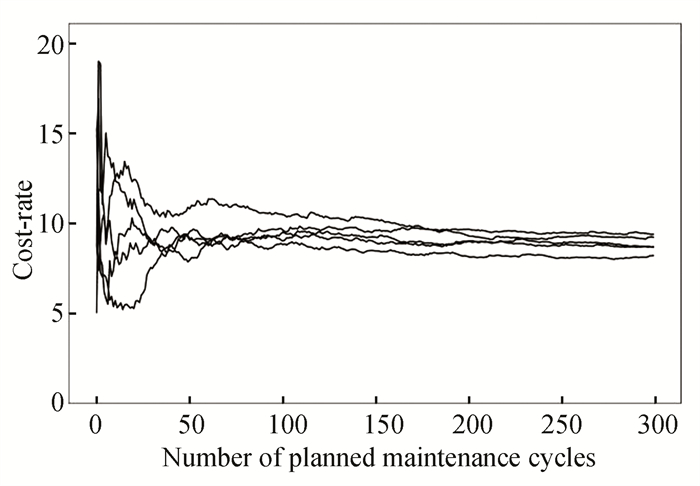
Firstly, to prove the convergence of the cost-rate, a simulation-analysis method is used by supposing T=40 and R0=0.6. To eliminate the chance of the simulation results and make it more convincing, the simulation is repeated five times. The result is shown in Fig. 7. It shows when the planned maintenance period number is big enough, five curve difference is small enough. So, it can infer the cost-rate is convergent when planned maintenance period number is big enough.
|
Fig.7 Cost-rate convergence based on proposed strategy |
After cost-rate is proved to be convergent, the following is to obtain the optimal solutions of the cost-rate by using the GA solver in the global optimization package of software R. The GA's parameters are set to 50 for the initial possible solutions, 0.05 for the uniform mutation probability, 1 for the crossover probability, and 100 for the number of iterations. After 100 iterations, the optimal values are received, i.e., (T*, R0*)=(41.30, 0.60), and the minimal cost-rate is CR(41.30, 0.60)=8.99. Finally, the optimal strategy is obtained.
3.2 Optimal Strategy EvaluationOptimal strategy is evaluated based on system reliability and maintenance cost.
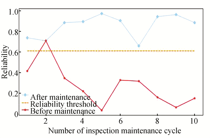
Firstly, to evaluate the impact of proposed strategy on system reliability, system reliability before and after maintenance is analyzed in the optimal case T*=41.30 and R0*=0.60, as shown in Fig. 8. The result shows that system reliability is significantly improved after system maintenance. This is because PM is triggered when system reliability is less than R0* at time Tr-. Afterwards, group importance measure will select Gz* for preventive replacement, which improves system reliability.
|
Fig.8 System reliability before and after maintenance |
Then, to verify the impact of the optimal maintenance strategy on maintenance cost, it is compared with another strategy[4]. Finally, the cost-rate analysis result is shown in Table 3. It shows the proposed strategy cost-rate is smaller than comparative strategy cost-rate. Because proposed strategy optimal PM maintenance period is less than that of the comparison strategy and the proposed strategy optimal reliability threshold is larger than that of the comparison strategy, this makes PM activities in the comparison strategy frequently executed. Finally, comparison result shows the proposed strategy can reduce maintenance costs by
| $ \frac{34.41-8.99}{34.41} \times 100 \%=73.87 \% $ |
| Table 3 Cost analysis of different strategies |
3.3 Sensitivity Analysis
Sensitivity analysis of cost parameters can summarize the impact of changes in cost parameters on cost-rate. To be precise, sensitivity analysis is to change the value of one cost parameter, while other cost parameters remain unchanged. In this section, let CR1(41.30, 0.60) be the proposed strategy cost-rate under T*=41.30 and R0*=0.60, and CR2(14.28, 0.56) be the comparative strategy cost-rate under T* = 14.28 and R0*=0.56, (as shown in Table 4). The sensitivity results of these four cost parameters are analyzed separately as follows:
| Table 4 Sensitivity analysis of cost parameters |
1) cinsp ranges from 0 to 20 with 5 cost unit increments while other parameters remain unchanged. When cinsp is higher, cost-rate is higher. However, the proposed strategy cost-rate is always lower than comparative strategy cost-rate. So, cinsp is positively related with two maintenance strategies, respectively.
2) cs ranges from 0 to 20 with 5 cost unit increments while other parameters remain unchanged. When cs increases, cost-rate from two strategies also increases, but comparative strategy increases relatively faster. This is because in the optimal PM period, the comparison strategy is relatively small, so that the comparative strategy must frequently execute PM, and ultimately the cost-rate increases relatively quickly.
3) cpsd ranges from 0 to 200 with 50 cost unit increments while other parameters remain unchanged. Based on Eq. (21), cpsd is saved maintenance cost owing to group Gz, which is positive or negative value. Obviously, the cost-rate saved by cpsd is a positive value for the proposed strategy, but the cost-rate saved by cpsd is a negative value for the comparative strategy. In other words, cpsd is positively related to the comparative strategy and is negatively related to the proposed strategy.
4) cusd ranges from 100 to 300 with 50 cost unit increments while other parameters remain unchanged. When cusd is higher, maintenance cost-rate is higher.So, cusd is positively related to two maintenance strategies, respectively.
4 ConclusionsFirstly, the proposed maintenance strategy introduces a stress-strength model to depict component failure process because of internal degradation and external shock, and the system dynamic SSR is obtained in combination with the survival signature. Compared with the system reliability based on internal degradation, the system dynamic SSR is more realistic. Then, applying system dynamic SSR to system maintenance, an SMRCR rule considering the system structure updating and a two-level PM rule considering the group importance are formulated. Finally, using numerical example shows that the proposed maintenance strategy can effectively increase system reliability and reduces maintenance cost by 73.87%.
AppendixTo better illustrate survival signature definition, this section takes the 10-component system shown in Fig. A1 as an example for detailed explanation, in which components "1" and "2" belong to the same type 1, and components "3", "4" and "9" belong to type 2, components "5" and "10" belong to type 3, and components "6", "7" and "8" belong to type 4. The results of the survival probability of the system are shown in Table A1, in which all rows with survival probability 0 and 1 in the table are deleted.

|
Fig.A1 10-component system reliability block diagram |
| Table A1 10-component system survival signature |
Take l1=2, l2=1, l3=0, l4=2 as examples to explain the results in Table A1. This situation indicates that two components of type 1 are all working properly, a component of three components of type 2 is working normally, two components of type 3 are faulty, two components of three components of type 4 are in normal operation. At this time, all possible results of the component state vector are
| $ \left(\begin{array}{l} 2 \\ 2 \end{array}\right)\left(\begin{array}{l} 3 \\ 1 \end{array}\right)\left(\begin{array}{l} 2 \\ 0 \end{array}\right)\left(\begin{array}{l} 3 \\ 2 \end{array}\right)=9 $ |
so
| $ \prod\limits_{k=1}^4\left(\begin{array}{c} m_k \\ l_k \end{array}\right)^{-1}=\frac{1}{9} $ |
In the 9 possible results, there are only two combinations that components "1", "2", "3", "6", "8" and components "1", "2", "3", "7", "8" are all working properly to make the system work, i.e.,
| $ \sum\limits_{x \in S_{l_1, \cdots, l_K}} \phi(x)=2 $ |
Finally, the result is
| $ \varPhi(2, 1, 0, 2)=\frac{1}{9} \times 2=\frac{2}{9} $ |
| [1] |
Nicolai R P, Dekker R. Optimal maintenance of multi-component systems: a review. Kobbacy K A H, Murthy D N P. Complex System Maintenance Handbook. London: Springer, 2008: 263-286.
(  0) 0) |
| [2] |
Nguyen K A, Do P, Grall A. Condition-based maintenance for multi-component systems using importance measure and predictive information. International Journal of System Science, 2014, 1(4): 228-245. DOI:10.1080/23302674.2014.983582 (  0) 0) |
| [3] |
Vu H C, Do P, Barros A. A stationary grouping maintenance strategy using mean residual life and the birnbaum importance measure for complex structures. IEEE Transactions on Reliability, 2016, 65(1): 217-234. DOI:10.1109/TR.2015.2455498 (  0) 0) |
| [4] |
Nguyen K A, Do P, Grall A. Multi-level predictive maintenance for multi-component systems. Reliability Engineering and System Safety, 2015, 144: 83-94. DOI:10.1016/j.ress.2015.07.017 (  0) 0) |
| [5] |
Chen Y J, Feng H L. Maintenance strategy of multicomponent system based on structure updating and group importance measure. Communications in Statistics - Theory and Methods, 2022, 51(9): 2919-2935. DOI:10.1080/03610926.2020.1784434 (  0) 0) |
| [6] |
Li H, Deloux E, Dieulle L. A condition-based maintenance policy for multi-component systems with Levy copulas dependence. Reliability Engineering & System Safety, 2016, 149: 44-55. DOI:10.1016/j.ress.2015.12.011 (  0) 0) |
| [7] |
Rasmekomen N, Parlikad A K. Condition-based maintenance of multi-component systems with degradation state-rate interactions. Reliability Engineering and System Safety, 2016, 148: 1-10. DOI:10.1016/j.ress.2015.11.010 (  0) 0) |
| [8] |
Lemoine A J, Wenocur M L. On failure modeling. Naval Research Logistics Quarterly, 1985, 32(3): 497-508. DOI:10.1002/nav.3800320312 (  0) 0) |
| [9] |
Birnbaum Z W. On a Use of the Mann-Whitney Statistic. https://digitalassets.lib.berkeley.edu/math/ucb/text/math_s3_v1_article-02.pdf.
(  0) 0) |
| [10] |
Caballé N C, Castro I T, Pérez C J, et al. A condition-based maintenance of a dependent degradation-threshold-shock model in a system with multiple degradation processes. Reliability Engineering and System Safety, 2015, 134: 98-109. DOI:10.1016/j.ress.2014.09.024 (  0) 0) |
| [11] |
Castro I T, Caballe N C, Perez C J. A condition-based maintenance for a system subject to multiple degradation processes and external shocks. International Journal of Systems Science, 2015, 46(9-12): 1692-1704. DOI:10.1080/00207721.2013.828796 (  0) 0) |
| [12] |
Caballé N C, Castro I T. Analysis of the reliability and the maintenance cost for finite life cycle systems subject to degradation and shocks. Applied Mathematical Modelling, 2017, 52: 731-746. DOI:10.1016/j.apm.2017.08.002 (  0) 0) |
| [13] |
Huang K, Mi J, Wang Z J. Inference about reliability parameter with gamma strength and stress. Journal of Statistical Planning and Inference, 2012, 142(4): 848-854. DOI:10.1016/j.jspi.2011.10.005 (  0) 0) |
| [14] |
Nadar M, Kızılaslan F, Papadopoulos A. Classical and Bayesian estimation of P (X < Y) for Kumaraswamy's distribution. Journal of Statistical Computation and Simulation, 2014, 84(7): 1505-1529. DOI:10.1080/00949655.2012.750658 (  0) 0) |
| [15] |
Alaa H A. Stress-strength reliability for general bivariate distributions. Journal of the Egyptian Mathematical Society, 2016, 24(4): 617-621. DOI:10.1016/j.joems.2016.01.005 (  0) 0) |
| [16] |
Gao J, An Z, Liu B. A dependent stress-strength interference model based on mixed copula function. Journal of Mechanical Science and Technology, 2016, 30(10): 4443-4446. DOI:10.1007/s12206-016-0909-8 (  0) 0) |
| [17] |
Coolen F P A, Coolen-Maturi T. Modelling Uncertain Aspects of System Dependability with Survival Signatures. Cham: Springer International Publishing, 2015: 19-34.
(  0) 0) |
| [18] |
Hajian-Hoseinabadi H. Reliability and component importance analysis of substation automation systems. International Journal of Electrical Power and Energy Systems, 2013, 49: 455-463. DOI:10.1016/j.ijepes.2010.06.012 (  0) 0) |
 2023, Vol. 30


