0 Introduction

As the skeleton of the main reflecting surface, the back frame structure is the most important part of a large radio telescope. Geometric parameters of the back frame structure, such as the size of the beam section, will directly affect the accuracy of the main reflecting surface. There are several methods for optimizing the cross section size of the back frame structure^[1]. The first is the homologous design, whose main idea is that the back frame structure deforms under the load of its own weight. First the best matching paraboloid of the deformed reflecting surface is found. Then the best matching paraboloid is set as the deformed reflecting surface and thus the displacement value of each point on the reflecting surface is calculated. Finally, the beam cross-section is optimized until the deformation of the telescope structure meets the displacement value. In 1967 von Hoerner^[2] proposed the concept of homologous design. Chen^[3] proposed the accurate homologous design, in which the relative precision of reflecting surface can reach the extreme by satisfying the relative error of the reflective surface with zero RMS. The second method is to use the optimization module of general finite element software, in which RMS value can be directly used as the objective and the cross-section size of the beam as the design variable during the optimization of the back frame structure^[4]. The new search direction is determined by gradient calculation, and the linear search is used to minimize objective function in the module. However, this method requires continuous analysis of the first derivative information of the objective function, and the calculation workload is heavy. The third method is to use genetic algorithm as the optimization method. For example, Liu Yan et al. ^[5] introduced genetic algorithms in the cross-section optimization of the Xinjiang 110m all-movable telescope, and improved the electrical performance of the telescope.

Essentially, the telescope back frame structure optimization is the optimization of the truss^[6-7]. In terms of truss optimization, the full stress method is widely used^[8-9], in which the full stress criterion is applied to adjust the size of the section so that each beam can provide full response to its load-bearing performance and reach the full stress state. Although this kind of method cannot use the RMS value as the direct objective function and may not be able to obtain the best RMS, it still provides a new thought.

Aiming at the optimization problem of the back frame structure of the large radio telescope, an optimization criterion is derived based on the Lagrangian multiplier method and Kuhn-Tucker condition^[10]. Although this method does not take the RMS of the back frame as the direct optimization objective, it can guarantee the uniformity of the overall deformation of the structure. Comparison with the optimization results obtained by the first-order optimization method shows that the algorithm has a good optimization effect.

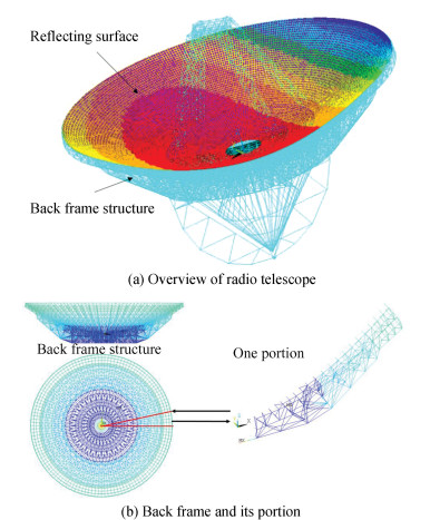
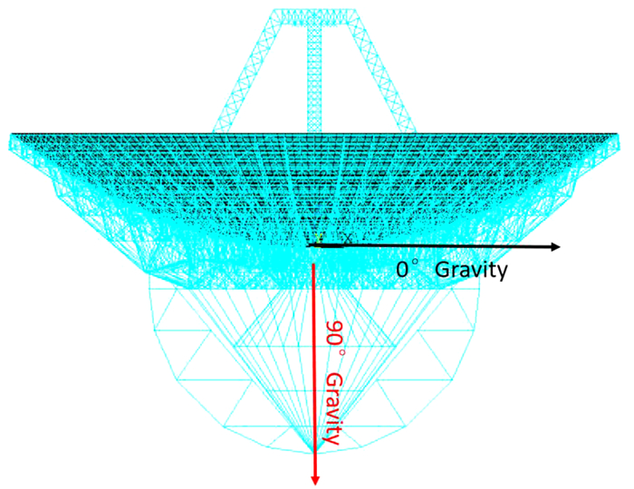
The back frame structure of a large radio telescope is complicated, but from a design point of view, the back frame is a rotationally symmetric structure composed of 32 identical portions^[11-13], as shown in Fig. 1. So optimization is only needed for one of them. There are 371 beams in one portion, whose inner and outer diameter are taken as the design variables. The optimal load case is 90° gravity, as shown in Fig. 2.

1 Back Frame Optimization Based on Optimization Criterion

In this section, based on the Lagrangian multiplier method, Kuhn-Tucker condition and finite element theory, a mathematical model is established using the beam inner and outer radiuses as design variables, the back frame compliance as constraint and the back frame volume as objective. And the section size optimization criterion is deduced from the model.

1.1 Optimization Mathematical Model

The mathematical model for back frame structure section size optimization is shown in Eq.(1).

$ \begin{aligned} & \text { find } \boldsymbol{R}=\left(r_{1, 1}, r_{1, 2}, r_{2, 1}, r_{2, 2}, r_{i, j}, \cdots, r_{n, 1}, r_{n, 2}\right) \\ & \min C(\boldsymbol{R})=\boldsymbol{U}^{\mathrm{T}} \boldsymbol{K} \boldsymbol{U}=\sum\limits_{i=1}^{n} \boldsymbol{u}_{i}^{\mathrm{T}} \boldsymbol{k}_{i} \boldsymbol{u}_{i} \\ & \text { s.t. } \quad \boldsymbol{K} \boldsymbol{U}=\boldsymbol{F}, i=1, 2, \cdots, n ; j=1, 2 \\ & \\ & \qquad \begin{array}{l} V=\sum\limits_{i=0}^{n} \pi\left(r_{i, 2}^{2}-r_{i, 1}^{2}\right) l_{i} \leqslant V^{*} \\ r_{\text {min }} \leqslant r_{i, 1} <r_{i, 2} \leqslant r_{\max } \end{array} \end{aligned} $

(1)

where r_{i, 1} and r_{i, 2} are the inner and outer radius of beam i; l_i is the length of beam i; R is a vector formed by all beams' section radius; n is the number of beams; V, C are the volume and compliance of the back frame structure; F is the force vector of the back frame structure; $\boldsymbol{U}, \boldsymbol{K}, \boldsymbol{u}_{i}, \boldsymbol{k}_{i}$ are the displacement and stiffness matrix of the structure of beam i respectively; V^* is the volume constraint; r_min and r_max are the limits of the section radius value.

1.2 Derivation of Optimization Criterion

Lagrange function of mathematical model Eq.(1) is shown in Eq.(2).

$ L=C+\boldsymbol{\lambda}_{1}^{\mathrm{T}}(\boldsymbol{K} \boldsymbol{U}-\boldsymbol{F})+\mu_{1}\left(V-V^{*}+x_{1}^{2}\right)+ \\ \sum\limits_{i=1}^{n} \mu_{2}\left(r_{\min }-r_{i, 1}+x_{2}^{2}\right)+ \\ \sum\limits_{i=1}^{n} \mu_{3}\left(r_{i, 1}-r_{i, 2}+x_{3}^{2}\right)+\sum\limits_{i=1}^{n} \mu_{4}\left(r_{i, 2}-\right. \\ \left.r_{\max }+x_{4}^{2}\right) $

(2)

where, $\boldsymbol{\lambda}_{1}, \mu_{1}, \mu_{2}, \mu_{3}, \mu_{4}$ are the Lagrange multipliers, $\boldsymbol{\lambda}_{1}$ is vector, $\mu_{1}, \mu_{2}, \mu_{3}, \mu_{4}$ are scalars, x₁, x₂, x₃, x₄ are slack variables.

Eq. (13) should satisfy the following Kuhn-Tucker condition, when $\boldsymbol{R}$ gets its extreme value.

$ \left\{\begin{array}{l} \frac{\partial L}{\partial r_{i, j}}=\frac{\partial C}{\partial r_{i, j}}+\boldsymbol{\lambda}_{1}^{\mathrm{T}} \frac{\partial K U}{\partial r_{i, j}}+\mu_{1} \frac{\partial V}{\partial r_{i, j}}+ \\ \quad\left\{\begin{array}{l} \mu_{3}-\mu_{2}(j=1) \\ \mu_{4}-\mu_{3}(j=2) \end{array}=0\right. \\ \boldsymbol{K} \boldsymbol{U}=\boldsymbol{F} \\ \mu_{1}\left(V-V^{*}\right)=0, \mu_{1} \geqslant 0, i=1, 2, \ldots, n, j=1, 2 \\ \mu_{2}\left(r_{\min }-r_{i, 1}\right)=0, \mu_{2} \geqslant 0 \\ \mu_{3}\left(r_{i, 1}-r_{i, 2}\right)=0, \mu_{3} \geqslant 0 \\ \mu_{4}\left(r_{i, 2}-r_{\text {max }}\right)=0, \mu_{4} \geqslant 0 \end{array}\right. $

(3)

For different values of design variable, $\boldsymbol{R}$, the Kuhn-Tucker condition Eq.(3) can be rewritten as:

$ \left\{\begin{array}{l} \frac{\partial L}{\partial r_{i, j}}=\frac{\partial C}{\partial r_{i, j}}+\boldsymbol{\lambda}_{1}^{\mathrm{T}} \frac{\partial \boldsymbol{K} \boldsymbol{U}}{\partial r_{i, j}}+ \\ \mu_{1} \frac{\partial V}{\partial r_{i, j}}\left\{\begin{array}{l} >0, \quad r_{i, 1}=r_{\text {min }} \\ <0, \quad r_{i, 2}=r_{\max } \\ =0, \quad r_{\min } <r_{i, 1} <r_{i, 2} <r_{\text {max }} \end{array}\right. \\ \boldsymbol{K} \boldsymbol{U}=\boldsymbol{F} \\ \mu_{1}\left(V-V^{*}\right)=0, \mu_{1} \geqslant 0 \end{array}\right. $

(4)

where i=1, 2, …, n; j=1, 2. When $\boldsymbol{R}$ gets to the extreme value, equation $\frac{\partial L}{\partial r_{i, j}}=0$ should be satisfied.

$ \frac{\partial L}{\partial r_{i, j}}=\frac{\partial C}{\partial r_{i, j}}+\boldsymbol{\lambda}_1^{\mathrm{T}} \frac{\partial \boldsymbol{K} \boldsymbol{U}}{\partial r_{i, j}}+\mu_1 \frac{\partial V}{\partial r_{i, j}}=0 $

(5)

Substitute $C=\boldsymbol{U}^{\mathrm{T}} \boldsymbol{K} \boldsymbol{U}$ into Eq.(5).

$ \begin{array}{r} \frac{\partial L}{\partial r_{i, j}}=\frac{\partial \boldsymbol{U}^{\mathrm{T}}}{\partial r_{i, j}} \boldsymbol{K} \boldsymbol{U}+\boldsymbol{U}^{\mathrm{T}} \frac{\partial \boldsymbol{K}}{\partial r_{i, j}} \boldsymbol{U}+\boldsymbol{U}^{\mathrm{T}} \boldsymbol{K} \frac{\partial \boldsymbol{U}}{\partial r_{i, j}}+ \\ \boldsymbol{\lambda}_{1}^{\mathrm{T}} \frac{\partial \boldsymbol{K}}{\partial \mathrm{r}_{\mathrm{i}, \mathrm{j}}} \boldsymbol{U}+\boldsymbol{\lambda}_{1}^{\mathrm{T}} \boldsymbol{K} \frac{\partial \boldsymbol{U}}{\partial r_{i, j}}+\mu_{1} \frac{\partial V}{\partial r_{i, j}}=0 \end{array} $

(6)

Considering the symmetry of the stiffness matrix, Eq.(7) and Eq.(8) can be obtained.

$\boldsymbol{U}^{\mathrm{T}} \boldsymbol{K} \frac{\partial \boldsymbol{U}}{\partial r_{i, j}}=\left(\boldsymbol{U}^{\mathrm{T}} K \frac{\partial \boldsymbol{U}}{\partial r_{i, j}}\right)^{\mathrm{T}}=\frac{\partial \boldsymbol{U}^{\mathrm{T}}}{\partial r_{i, j}} \boldsymbol{K} \boldsymbol{U} $

(7)

$ \boldsymbol{\lambda}_1^{\mathrm{T}} \boldsymbol{K} \frac{\partial \boldsymbol{U}}{\partial r_{i, j}}=\left(\boldsymbol{\lambda}_1^{\mathrm{T}} \boldsymbol{K} \frac{\partial \boldsymbol{U}}{\partial r_{i, j}}\right)^{\mathrm{T}}=\frac{\partial \boldsymbol{U}^{\mathrm{T}}}{\partial r_{i, j}} \boldsymbol{K} \boldsymbol{\lambda}_1 $

(8)

Then substitute Eq.(7) and Eq.(8) into Eq.(6).

$\begin{aligned} \frac{\partial L}{\partial r_{i, j}}= & \frac{\partial \boldsymbol{U}^{\mathrm{T}}}{\partial r_{i, j}}\left(2 \boldsymbol{K} \boldsymbol{U}+\boldsymbol{K} \boldsymbol{\lambda}_1\right)+ \\ & \left(\boldsymbol{U}^{\mathrm{T}}+\boldsymbol{\lambda}_1^{\mathrm{T}}\right) \frac{\partial \boldsymbol{K}}{\partial r_{i, j}} \boldsymbol{U}+\mu_1 \frac{\partial V}{\partial r_{i, j}}=0 \end{aligned} $

(9)

$\boldsymbol{\lambda}_{1}$ can take arbitrary value since it is the Lagrange multiplier for the structure equilibrium constraint and the structure equilibrium is always satisfied. Substitute $\boldsymbol{\lambda}_{1}=-2 \boldsymbol{U}$ into Eq.(9).

$ \frac{\partial L}{\partial r_{i, j}}=-\boldsymbol{U}^{\mathrm{T}} \frac{\partial \boldsymbol{K}}{\partial r_{i, j}} \boldsymbol{U}+\mu_1 \frac{\partial V}{\partial r_{i, j}}=0 $

(10)

That is,

$-\boldsymbol{u}_{i}^{\mathrm{T}} \frac{\partial k_{i}}{\partial r_{i, j}} \boldsymbol{u}_{i}+\mu_{1} \frac{\partial \boldsymbol{v}_{i}}{\partial r_{i, j}}=0 $

(11)

Considering the finite element theory, the partial derivatives of link element stiffness matrix $\boldsymbol{k}_{i}$, volume $\boldsymbol{v}_{i}$ can be written as:

$ \frac{\partial \boldsymbol{k}_{i}}{\partial r_{i, 1}}=-\frac{2 \pi r_{i, 1}}{A_{i}} \boldsymbol{k}_{i} $

(12)

$ \frac{\partial \boldsymbol{k}_{i}}{\partial r_{i, 2}}=\frac{2 \pi r_{i, 2}}{A_{i}} \boldsymbol{k}_{i} $

(13)

$\frac{\partial v_i}{\partial r_{i, 1}}=\pi l_i \frac{\partial\left(r_{i, 2}^2-r_{i, 1}^2\right)}{\partial r_{i, 1}}=-2 \pi l_i r_{i, 1} $

(14)

$ \frac{\partial v_i}{\partial r_{i, 2}}=\pi l_i \frac{\partial\left(r_{i, 2}^2-r_{i, 1}^2\right)}{\partial r_{i, 2}}=2 \pi l_i r_{i, 2} $

(15)

Therefore, Eq.(11) can be reduced to:

$ \begin{aligned} & \frac{2 \pi r_{i, 1}}{A_{i}} \boldsymbol{u}_{i}^{\mathrm{T}} \boldsymbol{k}_{i} \boldsymbol{u}_{i}-2 \mu_{1} \pi l_{i} r_{i, 1}=0, j=1 \\ & -\frac{2 \pi r_{i, 2}}{A_{i}} \boldsymbol{u}_{i}^{\mathrm{T}} k_{i} \boldsymbol{u}_{i}+2 \mu_{1} \pi l_{i} r_{i, 2}=0, j=2 \end{aligned} $

(16)

That is

$ \boldsymbol{u}_{i}^{\mathrm{T}} \boldsymbol{k}_{i} \boldsymbol{u}_{i}-\mu_{1} l_{i} A_{i}=0 $

(17)

where $\boldsymbol{u}_{i}^{\mathrm{T}} \boldsymbol{k}_{i} \boldsymbol{u}_{i}=2 e_{i}$, and $e_{i}$ is the strain energy of beam i, namely:

$ f_{i}=\frac{2 e_{i}}{\mu_{1} v_{i}}=1 $

(18)

Eq.(18) is the deduced section size optimization criterion for back frame structure. Using f_i as iterative criterion, the iterative equation of beam section radius can be obtained.

$r_{i, j}^{(k+1)}= \begin{cases}\left(f_{i}^{(k)}\right)^{\delta} r_{i, j}^{(k)} & , r_{\min } <\left(f_{i}^{(k)}\right)^{\delta} r_{i, j}^{(k)} <r_{\max } \\ r_{\text {min }}, & \left(f_{i}^{(k)}\right)^{\delta} r_{i, j}^{(k)} \leqslant r_{\min } \\ r_{\text {max }}, & \left(f_{i}^{(k)}\right)^{\delta} r_{i, j}^{(k)} \geqslant r_{\text {min }}\end{cases} $

(19)

where δ is a damping factor to insure convergence.

1.3 Optimization Results of Back Frame

The optimization parameters are shown in Table 1. $r_{i, 1}^{(0)}$ and $r_{i, 2}^{(0)}$ are the initial radiuses of the back frame beams. r_min and r_max are the limits of the radius value. w^* is the weight constraint which can be converted to volume constraint by dividing the density.

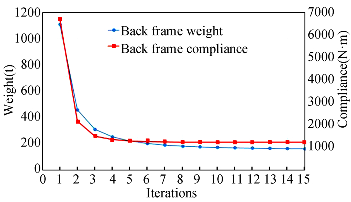
The variation curves of the back frame structure weight (constraint condition) and compliance (objective) during the optimization process is shown in Fig. 3. Curves show that this method has good convergence.

After optimization, the beams of back frame are divided into 6 categories, and the corresponding cross-section parameters of one portion are shown in Table 2.

2 Back Frame Optimization Based on First-Order Optimization Algorithm

The process of using first-order algorithm to optimize the section size of the back frame is shown in Fig. 4. The back frame structure is analyzed first. Then the back frame beams are divided into several categories according to the calculated stress. The cross-section parameters of each type are used as a set of design variables. Finally, the optimization design is carried out based on the above classification.

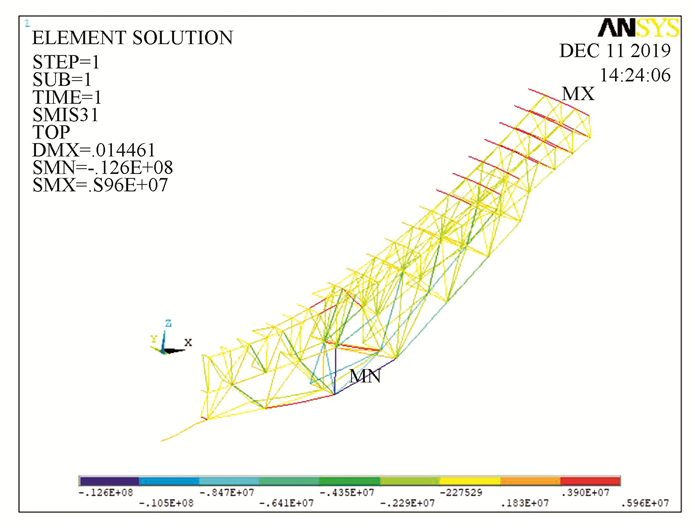
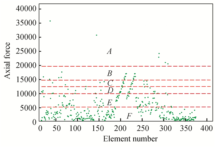
Fig. 5 shows the stress contour of a portion of the back frame after initial analysis. According to the stress in the beams, the beams are divided into 6 categories, as shown in Fig. 6 and Table 3. After the beams are classified, the inner and outer radiuses of each category of beam are used as design variables. So there are 6 sets of design variables, and each set has 2 design variables.

The mathematic model of first-order algorithm is showing in Eq.(20). In the equation, $\boldsymbol{R}$ is a vector composed of the above 6 sets of design variables. RMS is the root mean square error of the reflecting surface. W is the weight of back frame structure. W^* is weight constraint whose value is 150 t. The optimization initial value of $\boldsymbol{R}$ is shown in Table 3.

$ \mathrm{find}~~ \boldsymbol{R}=\left(r_{1, 1}, r_{1, 2}, r_{2, 1}, r_{2, 2}, \cdots, r_{i, j}, \cdots, r_{n, 1}, r_{n, 2}\right)\\ \min f=\mathrm{RMS} \\ \mathrm{s.t}. ~~ W <W^{*}\\ r_{\text {min }} \leqslant r_{i, 1} <r_{i, 2} \leqslant r_{\text {max }} $

(20)

First, rewrite the mathematic model as an unconstrained and dimensionless objective function, as shown in Eq.(21).

$ Q(\boldsymbol{R}, q)=\frac{f}{f_{0}}+\sum\limits_{i=1}^{n} P_{r}\left(r_{i}\right)+q P_{W}(W) $

(21)

where, f₀ is the reference value of objective. P_r(r_i) and P_W(W) are the penalty function of design variables and constraint which take the following form as shown in Eqs.(22)-(24).

$ P_{r}\left(r_{i}\right)=\left(\frac{r_{i}}{r_{i \text { upper }}+\alpha_{i}}\right)^{2 \lambda} $

(22)

$ P_{r}\left(r_{i}\right)=\left(\frac{r_{i \text { lower }}-\alpha_{i}}{r_{i}}\right)^{2 \lambda} $

(23)

$ P_{W}(W)=\left(\frac{W}{W_{0}+\beta}\right)^{2 \lambda} $

(24)

where λ is a large positive integer, α_i and β are very small positive number. So, when the constraint is broken, the penalty function will be very large. On the contrary, when the constraint condition is met, the penalty function value is smaller.

When carrying out optimization for the unconstrained and dimensionless objective function Eq.(21), a search direction vector $\boldsymbol{d}^{(j)}$ should be given in each optimization iteration to update the design variables, as shown in Eq.(25). The search direction vector $\boldsymbol{d}^{(j)}$ is calculated by the method of difference approximation, as shown in Eq.(26).

$ \boldsymbol{R}^{(j+1)}=\boldsymbol{R}^{(j)}+s_{j} \boldsymbol{d}^{(j)} $

(25)

$\frac{\partial Q\left(\boldsymbol{R}^{(j)}\right)}{\partial r_i}=\frac{Q\left(\boldsymbol{R}^{(j)}+\Delta r_i \boldsymbol{e}\right)-Q\left(\boldsymbol{R}^{(j)}\right)}{\Delta r_i} $

(26)

When $\boldsymbol{d}^{(j)}$ is determined, the step factor $\boldsymbol{s}_{j}$ can be calculated by a one-dimensional search algorithm.

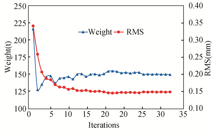
The variation curves of back frame structure weight (constraint condition) and RMS (objective) during the first-order optimization process is shown in Fig. 7. And the cross-section parameters of the beams after optimization and rounding are shown in Table 4.

3 Comparisons of Optimization Results of Two Methods 3.1 Back Frame Weight and RMS

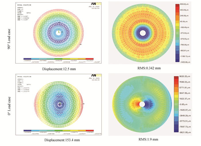
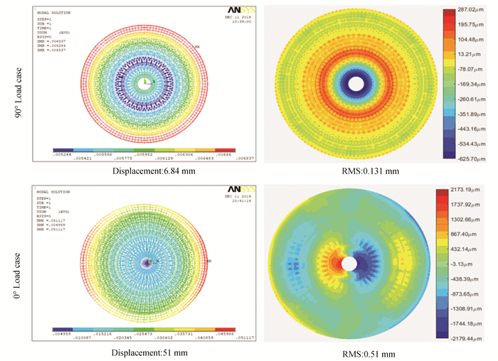
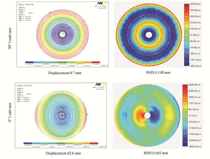
Comparison of the result of the original structure before optimization with the optimized results of the two methods (as shown in Table 5) shows that both optimization methods have obtained better optimization results. However, the results obtained by criterion method are noticeably better than those obtained by the first-order algorithm. The displacement contour and RMS contour before and after optimization are shown in Figs. 8-10.

3.2 Stress Distribution

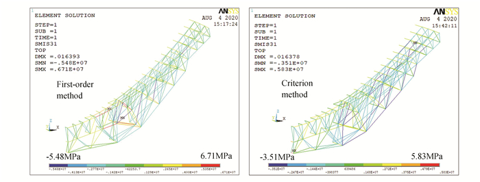
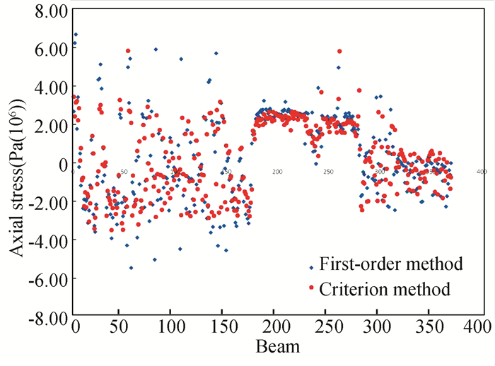
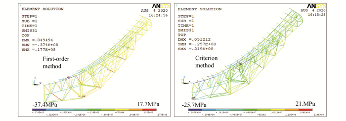
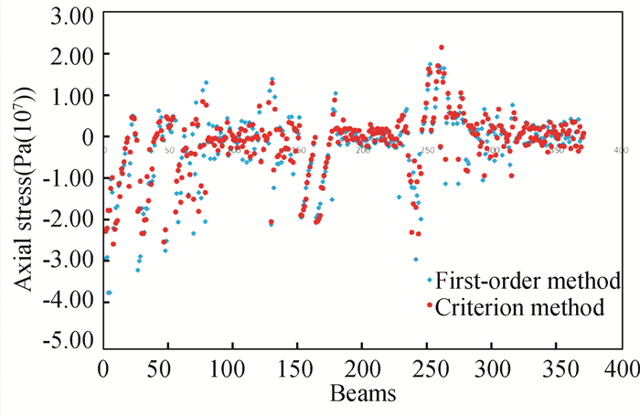
The stress contours and scatter plot of a portion of the back frame after the two optimization methods for 90°and 0°load cases, are extracted. The stress contour and scatter plot of the 90° gravity load case are shown in Figs. 11-12. It can be seen that the stress distribution of the back frame structure optimized by the first-order method is -5.48MPa-6.71MPa. Meanwhile the structural stress distribution optimized by criterion method is -3.51MPa-5.83MPa. The stress contour and scatter plot of 0° gravity load case are shown in Figs. 13-14. The corresponding two kinds of stress distribution are -37.4MPa-17.7MPa and -25.7MPa- 21.9MPa. Hence, it is obvious that the stress of the back frame structure optimized by the criterion method is more uniform.

3.3 Computational Efficiency

When using first-order method to carry out optimization design, in each iteration, gradient calculation is required to determine the search direction, and line search method is utilized to minimize the unconstrained problem. So, each iteration has a series of sub-iterations (including search direction and step length calculation), resulting in a heavy calculation workload when using the first-order optimization algorithm. The calculation time of first-order method is about 5 h. In the criterion method, the optimization direction has been given by the criterion, thus the optimization efficiency is high, which only takes an average of 20 min. Therefore, compared with the first-order method, the criterion method greatly improves the calculation efficiency.

4 Conclusions

The back frame structure of a large radio telescope is a skeleton that carries the reflecting surface, and its deadweight load has a great influence on the precision of the reflecting surface. In this paper, based on deadweight load case of the radio telescope, a section size optimization model is established, and optimization criterion is derived. At the same time, the first-order optimization algorithm is used for optimization comparison. The results show that both methods can achieve good optimization results. The optimized back frame has a lighter weight and higher RMS precision. In addition, the criterion method is determined to be better than the first-order method, including better RMS, more uniform structural stress and higher optimization efficiency.