With the increasing development of economy and urbanization, the phenomenon of job-housing separation has become prominent during the past few decades, which leads to a rapid increase in the number of automobiles on the road[1]. Especially during peak travel periods, there is a lot of commuting or return travel, leading to increased traffic congestion and pollution. In reality, automobile users always travel for various purposes. Therefore, many scholars have classified the purpose of travel, and studies on the analysis of trip purpose have emerged[2]. For instance, Gong et al.[3] divided taxi trips into 9 categories, which include Work-related, Transportation transfer and Schooling, etc. In addition, public transport trip purposes were assigned to Work, Education, Shopping, Home and Recreational based on smart card fare data[4]. As the road resources required for different trip purposes are quite different, and for some travel demands, public transport can be used to replace the use of automobiles[5]. Therefore, it is essential to effectively identify the trip purpose of traveler, rationalize the control of road traffic demand and transfer it to public transportation, which is regarded as resource-saving and environment-friendly mode of travel[6]. The above analysis indicates that exploring the trip purposes of automobile users is important for urban travel structure optimization and traffic demand management.
Trip purpose information is critical to human mobility analytics, which is a key component of travel behavior research. Generally speaking, the identification of trip purpose is often based on questionnaire data[7], GPS data[8-9], Automatic Fare Collection (AFC) data and bus IC card data[10], etc. However, questionnaires are always affected by both the investigators and the respondents. Especially when filling out the questionnaires, the respondents are always based on their vague memories and strong subjective preferences. Meanwhile, insufficient sample size will also cause systematic errors in the analysis results. Similarly, it is difficult to obtain GPS data on a large number of private automobile users, which usually involves the privacy of the travelers. IC card data and AFC data are usually only used to analyze the purpose of public transport travelers. Due to the difficulty of obtaining relevant data, there are few studies focusing on the trip purposes of automobile users. The advances in ever-increasing market penetration of traffic monitoring devices enabled generation of massive spatiotemporal trajectory data that capture automobile mobility patterns. Nevertheless, travelers through monitoring devices usually do not specify their trip purposes, which makes traffic analysts unclear whether the recorded travel is commuting or flexible travel.
With the rise of computer and artificial intelligence, machine learning techniques have gained increasing popularity due to their high accuracy in predicting simple as well as complex phenomena. Moreover, machine learning algorithms have been applied extensively to solve traffic and transportation problems due to their underlying precise and convenient mathematical models that can learn, generalize, and often reveal good predictive performance. Several researchers have shown the advantages of machine learning models, e.g., using Support Vector Machine (SVM)[11], Adaptive Boosting (Adaboost)[12] and Random Forest (RF)[13] can significantly improve the accuracy of model prediction. Meanwhile, in an experimental survey, it is found that RF is particularly suitable for the prediction of trip purposes[13]. Overall, the field of machine learning has received more and more attention in the research of travel behavior.
Based on the above analyses, our main objective in this paper is to mine the spatio-temporal characteristics of automobile trips and to classify and predict the purpose of automobile users by using road monitoring data. In our study, K-means clustering is used to divide the trip purposes of automobile users into four clusters, which include Commuting travel, Taxi travel, Flexible life demand travel in daytime and Evening entertainment and leisure shopping, respectively. Besides, AdaBoost and RF methods are used to predict the trip purpose of the preprocessed spatio-temporal dataset. Finally, the classification results are discussed after comparing and analyzing the two machine learning methods.
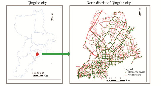
1 Multi-day Traffic Monitoring Data 1.1 Data Acquisition and ProcessingThis study conducts a case study of the Northern District of Qingdao, China. Qingdao is ranked as one of the top 15 cities by Gross Domestic Product (GDP) index in China. It has more than 3.55 million motor vehicles. Northern District is located in the south-central part of Qingdao with a total land area of 65.4 km2 and a population of around 1096879, which is one of the most important central areas. As shown in Fig. 1, the traffic monitoring devices in the North District of Qingdao are densely distributed, including about 1922 monitoring devices to facilitate real-time traffic flow management. Therefore, travel characteristics of automobiles can be obtained from traffic monitoring data to some extent. This paper contains traffic monitoring data from January 16 to January 22, 2022 in the Northern District of Qingdao, China.
|
Fig.1 Distribution of monitoring devices in Northern District of Qingdao |
Since the questionnaire data are always influenced by the respondents' own memory and preferences as well as the researchers' own preferences for selecting respondents. Multi-day traffic monitoring data are used to identify the attributes of automobile travel in the study area. Compared with the questionnaire data, the historical data can describe real vehicle travel characteristics. Therefore, we can use it to select effective and reasonable descriptive variables according to the actual travel structure proportion and features.
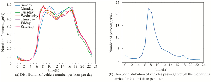
Monitoring devices record the relevant characteristics of the vehicle passing through, including license plate number, passing time, passing location, etc. The study collected a week's worth of vehicle records containing 25000000 pieces of data generated by approximately 1 million vehicles per day through monitoring devices. Fig. 2(a) shows the number of vehicles passing through the monitoring device in one day. From this figure, it can be seen that the traffic flow at morning and evening peaks is significantly larger than at other periods, and the traffic flow in the morning rush hour is slightly higher than that in the evening rush hour and establish six indicators from the data set: Time to first pass the monitoring device (e.g. Fig. 2(b) shows the number distribution of vehicles passing through the monitoring device for the first time per hour), Number of monitoring devices passed by automobiles, First trip time, Average daily trips, Number of travel days on working days and Number of days with the same destination for the first trip, respectively(Table 1). Then, the K-means clustering method is used to analyze data sets and classify vehicle data into several categories[14]. Meanwhile, two evaluation indexes which include Sum of Squares due to Error (SSE) and Calinski-Harabasz Score (CH_Score) are used to analyze the optimal clustering number and clustering effect[15]. Finally, we can obtain the distribution proportion of various main trip purposes in the study area.
|
Fig.2 Characteristics of vehicle time distribution |
| Table 1 Description of selected Variables |
It is worth noting that due to the high density of equipment in the road network, the vehicles are divided into two trips by the interval of more than one hour between two adjacent monitoring devices after testing according to data characteristics and the actual situation. In particular, CH_Score is defined as an internal clustering evaluation index as follows [15]:
| $ \text { CH_Score }(k)=\frac{\operatorname{tr} B(k) /(k-1)}{\operatorname{tr} W(k) /(n-k)} $ | (1) |
In Eq. (1), n represents the number of clusters, k represents the current class, trB(k) denotes the trace of the between-clusters deviation matrix, trW(k) denotes the trace of within cluster deviation matrix. Therefore, the greater the CH_Score value represents the closer the cluster itself, the more dispersed between clusters, which is, better clustering results.
1.2 Data AnalysisFrom the processed spatio-temporal dataset, we can get the statistical characteristics of the aforementioned six variables (as shown in Table 2).
| Table 2 Descriptive statistics of each variable |
K-means clustering is one of the practical clustering algorithms, which is easy to implement with fast convergence rate and strong interpretability. The step is to pre-divide the data into K groups, randomly select K objects as the initial clustering center, and then calculate each object and each seed. The distance between the clustering centers is assigned to the nearest clustering center. The cluster center and the objects assigned to them represent a cluster. Each time a sample is assigned, the cluster center will be recalculated according to the existing objects in the cluster. This process will be repeated until a termination condition is satisfied. The termination condition can be that no (or minimum number) objects are redistributed to different clusters, no (or minimum number) cluster centers change again, and the error sum of squares is locally minimal.
Therefore, based on the six variables mentioned above, K-means clustering is used in this study for classification to complete the preliminary analysis of the purpose of the trip. Due to the lack of description of data labels in unsupervised learning methods, two internal indicators (SSE and CH_Score) are used to evaluate the clustering effect in this paper. Meanwhile, the optimal number of clusters can also be obtained.
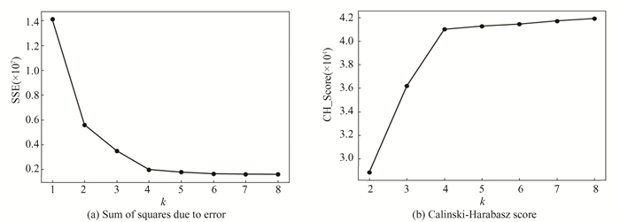
According to Fig. 3(a), with the increase of the number of clusters, SSE decreases gradually, and the curve tends to converge when k is close to 4. Meanwhile, CH_Score is also close to maximum when k = 4. Therefore, k = 4 can be selected as the best number of clusters in our work, and the clustering effect is best. The final clustering results are shown in Table 3.
|
Fig.3 Clustering performance results |
| Table 3 Final Clustering Centers |
As shown in Table 3, Cluster 1 has the largest number of vehicles and the least number of monitoring devices passed by vehicles, and the first time Cluster 1 passes through the monitoring device is almost during the morning peak hour, with an average daily trip of around 2. Apart from that, number of travel days on working days and number of days with the same destination for the first trip are close to 5, which basically conform to the commuter travel characteristic, so Cluster 1 can be divided into Commuting travel.
In particular, First trip time of Cluster 2 is much longer than others, which reaches almost 5 h (Due to the interval of 1 h in this study, taxis are usually cruising and parking time is short). Additionally, number of travel days on working days is close to 5 but its first destination varies greatly, which reflects that this category goes to different destinations every day. Consequently, Cluster 2 in this study is classified as taxi-based trips for other three types of purposes(hereinafter referred to as Taxi travel). Then, compared to Cluster 1, travelers in Cluster 3 usually avoid morning peak period (Such trips have relatively low requirements for departure time), the number of travel days on working days and number of days with the same destination for the first trip are slightly less than Cluster 1. Therefore, Cluster 3 can be regarded as Flexible life demand travel in daytime.
Interestingly, the characteristics of Cluster 4 are not obvious compared with the first three clusters. Overall, it looks similar to Cluster 3, but the biggest difference from the other three types is that the first travel time is in the evening. The time and space indicators cannot reach the characteristic of evening commuting. We can probably define it as Evening entertainment and leisure shopping travel.
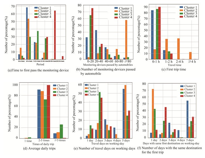
Moreover, in order to further explain the characteristics of the four types of trip purposes, the number distribution of variables in clustering results is shown in Fig. 4. Fig. 4(a) shows that the total proportion of first trips during 6-9 o'clock (morning peak hours) is significantly higher than during other periods, especially for commuting. Moreover, by combining Fig. 4(b) and Fig. 4(c), it can be found that the overall travel distance of the other three types of purposes is shorter except for taxi travel. In addition, Fig. 4(c)-4(f) magnifies the internal differences of various trip purposes from the time dimension and the spatial dimension. Commuting travel has strong temporal and spatial regularity, while elastic life travel and taxi are more random in temporal and spatial distribution.
|
Fig.4 Characteristics of four types of trip purpose |
In summary, the K-means clustering method is applied to divide the vehicles in the data set into four categories according to the purpose of travel. However, the clustering method is an unsupervised learning method, and only clustering method cannot further analyze the samples outside the data set [16]. In order to better study the trip purposes of automobile users, supervised learning algorithms are needed to mine intrinsic features in data. Therefore, the above clustering analysis can not only preliminarily analyze the trip purpose, but also provide data labels for subsequent classification prediction.
2 MethodologyOn the basis of applying K-means clustering to label the datasets in Section 1, the next step is to combine machine learning to find a classification method that can verify the characteristics of the most robust clustering results. In this section, two tree-based ensemble methods, AdaBoost and Random Forest method are applied in this paper for multi-class classification. The flowchart of trip purpose classification based on machine learning is shown in Fig. 5.
| $ G_m(x): X \rightarrow y_i \in Y, Y=\{-1, +1\} $ | (2) |

|
Fig.5 Flowchart of trip purpose classification based on machine learning |
2.1 AdaBoost
Boosting and bagging are the two major ensemble methods of the tree-based models. The boosting approach is an algorithm that trains the learners sequentially and assigns the weighting factor to each learner. As one of the typical boosting methods, adaptive boosting (AdaBoost) was first introduced by Freund and Schapire[17]. AdaBoost raises the weight of samples misclassified by weak classifiers in the previous round, reduces the weight of correct samples, and uses weighted majority voting to form a strong learner[12]. At first, all observations are weighted equally. Then, during the iterative training process, the observations which are incorrectly estimated by the learners will carry more weights. Therefore, this algorithm can iteratively adapt and reduce the deviation.
| $ \begin{gathered} e_m=P\left(G_m\left(x_i\right) \neq y_i\right)= \\ \sum\limits_{i=1}^n w_{m i} I\left(G_m\left(x_i\right) \neq y_i\right) \end{gathered} $ | (3) |
| $ \alpha_m=\frac{1}{2} \ln \frac{1-e_m}{e_m} $ | (4) |
| $ f_m(x)=\alpha_m G_m(x) $ | (5) |
Eq. (2) represents a basic classifier Gm(x) learned from a training dataset with weight distribution Dm=(wm1, wm2, …, wmn), m is the number of classifiers, and n represents the amount of data. em and αm are classification error rate and importance of the mth classifier, respectively(Eq. (3), Eq. (4)). Finally, a classifier with better performance fm(x) can be obtained in Eq. (5).
2.2 Random ForestThe bagging is a parallel learning process. For each round, a random subset of samples is drawn from the training sample randomly but with the same distribution. These selected samples are then used to grow a decision tree (weak learner) [18]. Then, the average prediction value is chosen as the final prediction value. Random forest method, as one of the most representative bagging methods, is used to predict trip purposes of automobile users in this subsection[19].
RF can train a distinctive decision tree corresponding to each training set with different structure. For each decision tree in the training process, the model will select the factors with the most classification ability as the splitting basis of the current decision node according to the Gini coefficient (Eq. (6) to Eq. (8)). Similarly, each sub-node will also be split according to the Gini coefficient. If the conditions for stopping splitting are met, the trip purpose with the largest proportion of the node is taken as the output result. By repeating the above process, a forest composed of F decision trees can be obtained. Each decision tree will give a predicted trip purpose of each traveler in the test set by inputting the influenced factors into the constructed forest in turn. And finally, the trip purpose result of traveler is predicted through the voting principle.
| $ {Gini}(E)=\sum\limits_{j=1}^J \sum\limits_{j^{\prime} \neq j} p_j p_{j^{\prime}}=1-\sum\limits_{j=1}^J p_j^2 $ | (6) |
| $ {Gini}(E, x)=\sum\limits_{h=1}^H\left|\frac{E_h}{E}\right| {Gini}\left(E_h\right) $ | (7) |
| $ x^*=\arg \;\min ({Gini}(E, x)), x \in X^{\prime} $ | (8) |
Eq. (6) represents the definition of Gini coefficient, which can be expressed as the purity of any dataset E. The purity of dataset E is negatively correlated with Gini(E), J represents the trip purposes of the dataset, and pj is the proportion of samples of class j over the total samples. Therefore, the Gini coefficient of the influencing factor x can be utilized as the basis for splitting at the decision junction, and the calculation procedure as shown in Eq. (7) and Eq. (8). Assuming that there are H possible values {x1, x2, ……, xH} for influencing factor x, H nodes will be generated if x is used to divide the data set. Eh represents the samples in the h-th branch node whose value is xh. Among all the influencing factors X', the factor x* that minimizes the Gini coefficient after division is selected as the optimal division attribute.
2.3 Model EvaluationAs non-parametric models, machine learning models cannot evaluate the performance of the model by maximum likelihood estimation. K-fold cross-validation based on the resampling method is widely used in model comparison [20]. The training set samples are divided into K equal parts, one of which is selected as the test, and the remaining K-1 are trained. The classification accuracy obtained from each cross-validation is recorded. And finally, the average value A is calculated as the final prediction accuracy of the model.
Due to the different model construction processes, different indicators and evaluation criteria are adopted to determine the most suitable machine learning model. In addition, when solving classification problems, we can also use common indicators (e.g., confusion matrix) to evaluate the effectiveness of classification[21]. Therefore, the confusion matrix is used to better represent comparison results, which compares the predicted with the observed behavior and reveals how incorrect predictions are distributed among the observed clusters. The analysis of this research was presented in two different perspectives: (a) training and testing results of the prediction accuracy by utilizing all features. (b) adjusting the relevant parameters of the model to train and test the results of the prediction accuracy.
3 Results and AnalysisThe empirical results are introduced in this section. Specifically, we select learning rate, maximum depth and number of trees as the representative hyper-parameters to compare the prediction accuracy of machine learning models. Meanwhile, how different prediction accuracy changes under various hyper-parameters is studied through simulation tests. Additionally, confusion matrix of two models is applied to compare prediction performance.
3.1 Model Development with K-fold Cross-validationA 5-fold cross-validation was implemented to train the AdaBoost and Random forest models. The cross-validation was to overcome the over-fitting issue and ensure the models' reliability in predicting trip purpose in a new dataset. The Mean Absolute Error (MAE), Root Mean Squared Error (RMSE), and R2 were used to assess the model performance. These measures, which could directly reflect the difference between the observations and predictions, have been widely employed for evaluating the model performance in machine learning studies. A tuning process was applied to determine the best set of parameters for each machine learning model, especially the maximum depth of trees and number of trees (equivalent to n_estimates below) to control the over-fitting of the RF as well as the learning rate and tree number for AdaBoost. The cross-validation training results and testing results of the two models are summarized in Table 4. The performance of both models is optimized with the increase of correlated hyper-parameter combination values. Besides, by comparing between two methods, it could be found that the MAE and RMSE of AdaBoot are smaller when the hyper-parameter is at a low value. It is clearly shown that the RF with larger hyper-parameters could gain better performance than AdaBoost for estimating trip purpose.
| Table 4 Results of 5-fold cross-validation |
3.2 Comparison of Model Performance
In order to determine the most accurate method for predicting trip purpose, AdaBoost and Random Forest, two methods with superior prediction ability, are further compared. The same training data and test data are used to train and evaluate these models.
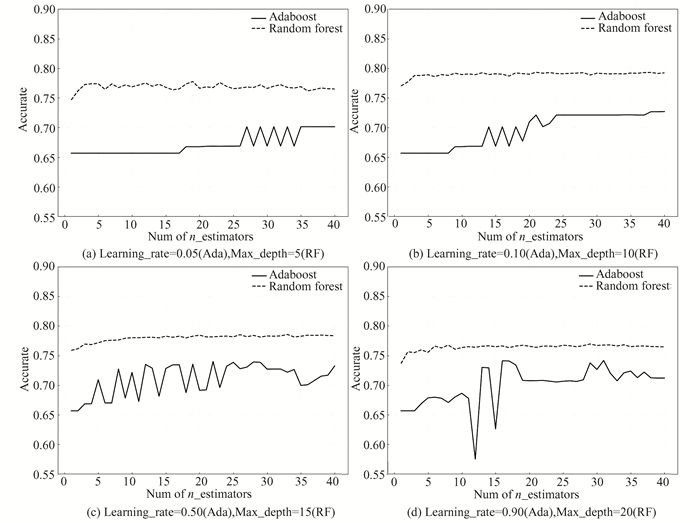
In general, as shown in Fig. 6, RF has higher prediction accuracy than AdaBoost, especially when the learning_rate and number of n_estimators are small, the prediction accuracy of Random Forest is significantly higher than that of AdaBoost. By contrast, the prediction accuracy of AdaBoost with different learning rates and n_estimators is unstable and fluctuates greatly under some parameter combinations.
|
Fig.6 Model accuracy under different hyper-parameters |
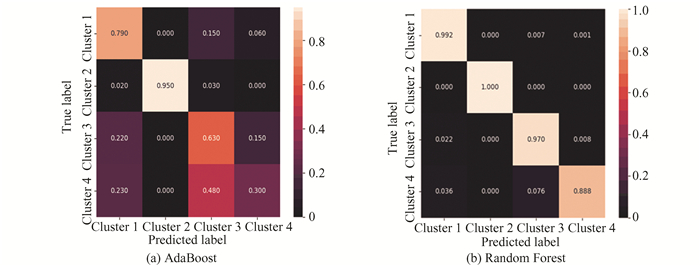
Fig. 7 shows the confusion matrix of two tree-based ensemble learning models. It can be concluded that RF is superior in predicting trip purpose, while the precision accuracy of AdaBoost is much lower, especially for the prediction of Cluster 4 (0.300 in Fig. 7(a)). It proves that RF can get more accurate results than AdaBoost in the prediction of trip purposes. Meanwhile, it also shows that the RF, to a certain extent, improves the applicability to the problem of trip purpose when using monitoring data.
|
Fig.7 Confusion matrix of two models |
Overall, in this section, two tree-based ensemble methods, RF and AdaBoost, are chosen to process road monitoring data. On the basis of K-means clustering, the classification and prediction of four types of trip purposes are compared and analyzed. After k-fold cross-validation of the two methods, the optimal parameters of the model are selected, and the applicability of the two models is tested under the same dataset. The results show that in this case, the classification prediction effect of random forest is better, which provides a reference for dealing with similar problems in the future.
4 Conclusions and RecommendationsDue to the complexity of automobile travel structure, the travel characteristics cannot be fully analyzed using GPS data or questionnaire data. In this paper, we choose road monitoring data with broader coverage to analyze the spatial and temporal characteristics of automobile trips. Focusing on K-means clustering and machine learning, this paper aims to classify and predict the trip purposes of automobile users. Our work can provide a basis for exploring the characteristics of urban automobile travel, and also provide suitable public transportation modes (such as demand-responsive bus, bus rapid transit and bus express) to replace automobile travel for different trip purposes, which can help optimize the urban road traffic structure and ensure the sustainable development of urban transportation system. The core ideas and important breakthroughs mainly include the following three parts:
(1) Traffic monitoring data, which have not been used in previous studies about trip purpose, are applied in our research, and the combination of supervised and unsupervised learning methods is verified to be effective in analyzing specific travel problems. This can not only analyze trip purpose from a new perspective, but also provide a great reference for future research on travel behavior.
(2) Based on the road monitoring dataset in Qingdao, six indicators were established to analyze the spatial and temporal characteristics of automobile user trips. Then, the K-means clustering method is used to analyze dataset and the purpose of automobile users in research area can be mainly divided into four categories according to the convergence value of SSE and CH_Score, which include Commuting trips, Flexible life demand travel in daytime, Evening entertainment and leisure shopping, and Taxi-based trips for the first three types of purposes, respectively. This allows us to indirectly understand the travel structure of automobile users, which can help traffic managers to implement different measures for different purposes.
(3) According to the result of K-means clustering, the prediction accuracy of two tree-based ensemble learning methods is analyzed from multiple aspects. It is found that random forest is more suitable for processing trip purpose prediction under hyper-parameter optimization. The values of MAE, RMSE and R2 are better than AdaBoost. In addition, the average prediction accuracy of RF can reach 96.25%, which is also higher than AdaBoost. It provides a reference for dealing with travel behavior problems.
To sum up, this study applies road monitoring data to analyze the trip purposes of automobile users from an indirect perspective, which provides a new research direction for applying machine learning to the study of travel behavior, but there is still room for improvement. In our research, Cluster 4 has lower prediction accuracy than other Clusters, which is mainly reflected in the greater distinction in evening trip purposes. This requires a more detailed description of evening travel. In the future, we will study more ensemble learning models to improve classification accuracy. In addition, although the amount of traffic monitoring data is large enough, the method of sampling analysis in our study will bring some errors, we will try to use a larger sample size to study the relevant problem. Future studies can also apply multi-source datasets including GPS and questionnaire data to improve research defects.
| [1] |
Xu C, Li H, Zhao J, et al. Investigating the relationship between jobs-housing balance and traffic safety. Accident Analysis and Prevention, 2017, 107: 126-136. DOI:10.1016/j.aap.2017.08.013 (  0) 0) |
| [2] |
Lu Y, Zhang L. Imputing trip purposes for long-distance travel. Transportation, 2015, 42(4): 581-595. (  0) 0) |
| [3] |
Gong L, Liu X, Wu L, et al. Inferring trip purposes and uncovering travel patterns from taxi trajectory data. Cartography & Geographic Information Science, 2016, 43(2): 103-114. DOI:10.1080/15230406.2015.1014424 (  0) 0) |
| [4] |
Alsger A, Tavassoli A, Mesbah M, et al. Public transport trip purpose inference using smart card fare data. Transportation Research Part C: Emerging Technologies, 2018, 87: 123-137. (  0) 0) |
| [5] |
Beaudoin J, Cynthia Lin Lawell C-Y. The effects of public transit supply on the demand for automobile travel. Journal of Environmental Economics and Management, 2018, 88: 447-467. DOI:10.1016/j.jeem.2018.01.007 (  0) 0) |
| [6] |
Yang W, Chen H, Wang W. The path and time efficiency of residents' trips of different purposes with different travel modes: an empirical study in Guangzhou, China. Journal of Transport Geography, 2020, 88: 102829. DOI:10.1016/j.jtrangeo.2020.102829 (  0) 0) |
| [7] |
Ramos É M S, Bergstad C J, Nssé J. Understanding daily car use: driving habits, motives, attitudes, and norms across trip purposes. Transportation Research Part F: Traffic Psychology and Behaviour, 2020, 38: 306-315. DOI:10.1016/j.trf.2019.11.013 (  0) 0) |
| [8] |
Byon Y J, Abdulhai B, Shalaby A. Impact of sampling rate of GPS-enabled cell phones on mode detection and GIS map matching performance. Transportation Research Board 86th Annual Meeting. Washington DC, 2007.
(  0) 0) |
| [9] |
Bohte W, Maat K. Deriving and validating trip purposes and travel modes for multi-day GPS-based travel surveys: a large-scale application in the Netherlands. Transportation Research Part C: Emerging Technologies, 2009, 17(3): 285-297. DOI:10.1016/j.trc.2008.11.004 (  0) 0) |
| [10] |
Jia N, Li L, Ling S, et al. Influence of attitudinal and low-carbon factors on behavioral intention of commuting mode choic-a cross-city study in China. Transportation Research Part A: Policy and Practice, 2018, 111: 108-118. DOI:10.1016/j.tra.2018.03.010 (  0) 0) |
| [11] |
Kim E J, Kim Y, Jang S, et al. Tourists' preference on the combination of travel modes under mobility-as-a-service environment. Transportation Research Part A Policy and Practice, 2021, 150: 236-255. DOI:10.1016/j.tra.2021.06.016 (  0) 0) |
| [12] |
Cai Q, Abdel-Aty M, Zheng O, et al. Applying machine learning and google street view to explore effects of drivers' visual environment on traffic safety. Transportation Research Part C: Emerging Technologies, 2022, 135: 103541. DOI:10.1016/j.trc.2021.103541 (  0) 0) |
| [13] |
Ermagun A, Fan Y, Wolfson J, et al. Real-time trip purpose prediction using online location-based search and discovery services. Transportation Research Part C: Emerging Technologies, 2017, 77: 96-112. DOI:10.1016/j.trc.2017.01.020 (  0) 0) |
| [14] |
Yang W, Long H, Ma L, et al. Research on clustering method based on weighted distance density and K-means. Procedia Computer Science, 2020, 166: 507-511. DOI:10.1016/j.procs.2020.02.056 (  0) 0) |
| [15] |
Gagolewski M, Bartoszuk M, Cena A. Are cluster validity measures (in) valid?. Information Sciences, 2021, 581: 620-636. DOI:10.1016/j.ins.2021.10.004 (  0) 0) |
| [16] |
Yu J J Q. Semi-supervised deep ensemble learning for travel mode identification. Transportation Research Part C: Emerging Technologies, 2020, 112(3): 120-135. DOI:10.1016/j.trc.2020.01.003 (  0) 0) |
| [17] |
Freund Y, Schapire R E. A decision-theoretic generalization of on-line learning and an application to boosting. Journal of Computer and System Sciences, 1997, 55(1): 119-139. DOI:10.1006/jcss.1997.1504 (  0) 0) |
| [18] |
Griffin T, Huang Y. A decision tree classification model to automate trip purpose derivation. Proceedings of the ISCA International Conference on Computer Applications in Industry & Engineering, Hnolulu: DBLP, 2005.
(  0) 0) |
| [19] |
Lu J, Meng Y, Timmermans H, et al. Modeling hesitancy in airport choice: a comparison of discrete choice and machine learning methods. Transportation Research Part A: Policy and Practice, 2021, 147: 230-250. DOI:10.1016/j.tra.2021.03.006 (  0) 0) |
| [20] |
Qi X, Wu G, Boriboonsomsin K, et al. Data-driven decomposition analysis and estimation of link-level electric vehicle energy consumption under real-world traffic conditions. Transportation Research, 2018, 64: 36-52. DOI:10.1016/j.trd.2017.08.008 (  0) 0) |
| [21] |
Fu T, Yu X, Xiong B, et al. A method in modeling interactive pedestrian crossing and driver yielding decisions during their interactions at intersections. Transportation Research Part F: Traffic Psychology and Behaviour, 2022, 88: 37-53. DOI:10.1016/j.trf.2022.05.005 (  0) 0) |
 2023, Vol. 30


