 2023, Vol. 30


2. Mechanical Engg. Dept., Annamacharya Institute of Technology and Sciences, Rajampet 516126, Andhara Pradesh, India;
3. Mechanical Engg. Dept., Mohan Babu University, A.Rangampet 517102, Andhra Pradesh, India;
4. Electronics and Communication Engg. Dept., Annamacharya Institute of Technology and Sciences, Tirupati 517520, Andhara Pradesh, India
Manufacturing businesses must deal with increasing product complexity, shorter market time, new technologies, global competitive concerns, and a rapidly changing environment. FMS is designed to compete in the manufacturing industry. FMS is a computer numerically controlled (CNC) integrated production system that includes multipurpose machine tools coupled to an automated material handling system (MHS)[1]. FMS strives for manufacturing flexibility without compromising product quality. The FMS depends on the flexibility of automated MHS, CNC machines, and control software to achieve its flexibility. Workflow patterns, size, and manufacturing type have all been used to group FMSs into different kinds. From a planning and control standpoint, there are four types of FMS: single flexible MCs (SFM), flexible manufacturing cells (FMC), multi-cell FMS (MCFMS), and multi-machine FMS (MMFMS)[2]. Existing FMS installations have confirmed benefits such as cost savings, increased utilization, and lower work-in-process[3]. Scheduling tasks improve resource utilization by lowering MSN[4]. Solving scheduling problems optimally or near optimally is one technique to attain high productivity in FMS.
Because of economic considerations, the number of tool copies is restricted, and there may be fewer of them than there are machines. This causes tool loading to be a hard part of scheduling challenges. A technical answer to the escalating tools' cost in FMS is an automated tool sharing system that enables several machines to use the same tool by automatically switching it from one to another machine (MC) by TT as tooling necessities change. Because FMS is a fully integrated manufacturing plant, it is critical to schedule all of its components simultaneously. The inability to effectively manage tool loading and job scheduling (shdng) can yield an underutilization of capital-intensive machinery and a significant amount of idle time. As a result, efficient job and tool shdng allows a production system to maximize MC utilization and reduce idle periods[5]. Much research has been undertaken on MCs and tools joint shdng simultaneously. Tang and Denardo[6] tackled the issue of figuring out the job order and tools that should be deployed before each job is executed on the MC to minimize tool changes. Chandra et al.[7] provided a practical method for determining the order of jobs and tools to reduce overall set-up and processing durations and ensure that jobs are finished on time. Song et al.[8] described a heuristic technique for assigning tools and parts to minimize tool swaps across MCs by requiring each part to process entirely on just one MC. In minimizing the overall tardiness by utilizing a tool movement plan where each component only wants to process entirely on just one MC in FMS, Roh and Kim[9] investigated the allocation of parts and tools as well as shdng issues. Agnetis et al.[1] tackled integrated part and tool shdng in FMC to minimize MSN and maximum delay by keeping tools in a CTM shared by MCs that utilize TT. The Tabu search approach is used to settle disputes when 2 MCs need the same tool. In addition to a method for sharing tools in FMS to cope with unexpected job introductions in a dynamic environment, a distributed artificial intelligence strategy for tool scheduling and borrowing issues was proposed by Tsukada and Shin[10]. It has been proved that sharing tools among different FMS cells reduces tooling costs and enhances tool use. Greedy Search Algorithm was advocated by Jun, Kim, and Suh[11] for shdng and delivering tools, as well as determining the number of new tools necessary when FMS configuration alters due to changes in the product mix to minimize MSN in the FMS. Keung, Ip, and Lee[12] examined tool switching scenarios and tool switches using a GA methodology to analyze MC allotment and job shop planning on a parallel machining workstation combined with several MCs that shared tools. On an SFM fixed with a tool magazine, where every job needs one of the tools, Ecker and Gupta[13] suggested a job precedence relationship algorithm. The objective of this algorithm was to arrange jobs to minimize the total amount of time necessary for tool changes. In the FMC with "m" work cells identical to the CTM, Prabaharan et al.[14] employed a preference dispatching rule and simulated annealing approaches to manage coupled operation shdng and a tool for MSN minimization. On SFM with a restricted tool magazine capacity, Karzan and Azizoǧlu[15] addressed the problem of job shdng and TT operations. A branch-bound algorithm and beam search approach provides the best possible or near ideal solutions for minimizing TT motions among the tool crib and MC region. Suresh Kumar and Sridharan[16] reported simulation research examining the influence of shdng restrictions on FMS component commence and tool appeal decisions. FMS was adhering to a guideline that included both tool and part movement. A simulation study is utilized to indicate the best combinations of shdng rules for component launch and tool demand selection for mean flow time, tardiness, and conditional mean tardiness minimization. Udhayakumar and Kumanan[17] proposed the Ant Colony Optimization Algorithm to build optimal job and tool orders to minimize MSN for FMS, and enhanced GT approaches were employed for active schedule development. Udhayakumar and Kumanan[18] advocated unconventional optimization strategies, including SA, GA, PSO, and ACO, to construct the optimal jobs and tools to minimize tardiness in FMS, and revised GT algorithms were put to use to produce effective schedules. Aldrin Raj et al.[19] offered four algorithms to determine MC and tool combination shdng in an FMS with 4 MCs and 1 CTM to reduce MSN. To minimize MSN, zpeynirci[20] proposed a time-indexed mathematical approach for MC and tool shdng in an FMS. Costa et al.[21] devised a hybrid GA that uses a local search improvement method to handle 'p' parts using 'q' MCs shdng considering tool alter activity prompted by tool wear. Reddy et al.[22-23] addressed MCs and tools joint scheduling in an MMFMS to provide the best optimum sequences with a single copy of every tool kind that minimizes MSN. Chaithanya et al.[24] discussed the cooperative MCs and tools joint shdng with a duplicate of each tool type to reduce MSN. They demonstrated that the Jaya algorithm outperforms the other ones currently in use. Beezao et al.[25] utilized an adaptive large neighborhood search metaheuristic to define and resolve the problem of indistinguishable parallel MCs with tooling restrictions for minimizing MSN (ALNS). It has been demonstrated that ALNS outperforms other current algorithms. Using the simulated annealing approach, Baykasoǧlu and Ozsoydan[26] tackled the indexing of automated tool changer (ATC) and tool changing problems simultaneously to minimize non-machining durations of automatic machining centers. Paiva and Carvalho[27] investigated the job sequence and tool changing issue (SSP) to determine the job sequence and tool loading order to reduce tool changes. An approach that uses heuristic methods, graph representation, and local search methods is applied for solving sequencing problems. These strategies are used with a traditional tools approach to solving SSP in an algorithmic local search method. To solve challenges with preset tool quantities in the system due to financial restrictions and minimize MSN, Gökgür et al.[28] employed constraint programming models in parallel MC configurations. In the references discussed above, job shipping periods and tool transport times among MCs are not considered, and operations are only scheduled on primary MCs.
Considering tool switch times amid MCs with a single copy of every tool kind (SMTTATWPM) for minimum MSN as an objective, Sivarami Reddy et al.[29-30] solved MCs and tools parallel shdng problems and demonstrated that tool shift times have a substantial impact on MSN. Operations are solely planned on specific MCs, and job travel times are not taken into account.
To locate the best sequences for minimization of MSN in MMFMS, Sivarami Reddy et al.[31-32] studied MCs, tools, and automated guided vehicles (AGVs) concurrent shdng with a single copy of each tool kind while considering job shift durations amongst MCs, without considering, and considering tool transport times among MCs, respectively. Padma Lalitha et al.[33] addressed machines, TT and tools simultaneous shdng in a multi machine flexible manufacturing system (FMS) with the lowest possible number of copies of every tool type without tool delay taking into account tool transfer times to minimize make span using crow search algorithm. Padma Lalitha et al.[34] tackled machines, AGVs and tools simultaneous shdng in a multi-machine flexible manufacturing system (FMS) with the lowest possible number of copies of every tool type without tool delay considering jobs' transport times among machines to minimize make span using SOSA.
In the above-examined references, the operations of different jobs are scheduled on primary MCs. When operations belong to different jobs needing the same MC, MC can be allocated to one operation only; therefore, other operations have to wait for the MC, which introduces MC delay. When alternate MCs are available, if one is busy, the other can be allocated to minimize MC delay. Therefore there is a reduction in MSN.
However, very few researchers addressed the shdng with alternative routing because of the complexity of the problem. Wilhelm and Shin[35] carried out a study to examine the alternative operations efficacy in FMSs. It has been shown through computational studies that alternative operations can decrease flow time while improving the utilization of MC. With alternative MC routings in a general job shop, Nasr and Elsayed[36] introduced an effective heuristic for mean flow time minimization. Moon and Lee[37] suggested a distinct GA representation for addressing the job shop's shdng issue through alternative routing. A differential evolution (DE) was presented by Satish Kumar et al.[38] for MCs and AGVs parallel shdng with alternative MCs. This DE included a heuristic for MC choice as well as a heuristic for vehicle allocation. Sivarami Reddy et al.[39-40] handled the problem of concurrent scheduling of MCs and tools with a single copy of each tool kind and alternate MCs (SMTWAM) by using the SOSA and the crow search algorithm to minimize MSN. They showed that using alternate MCs could reduce MSN. Time spent transferring jobs and tools amid MCs are not taken into account.
In the MCs and tools parallel shdng with a single copy of each tool kind considering tool shift durations among MCs (SMTTATWPM), the operations of different jobs are scheduled on primary MCs. When the same MC is required by operations of different jobs simultaneously, the MC can only be assigned to one operation. Therefore it causes other operations to wait for the MC, resulting in a MC delay. If one MC is busy, the other MC can be allocated so that the MC delay can be minimized when the operation can be processed on more than one MC, i.e., alternate MCs in SMTWAM. Therefore there is a reduction in the MSN. Tools are transferred by the TT among CTM and MCs and between the MCs. Therefore, shdng of TT is important in MCs, and tools combined shdng with alternate MCs, as tool shift times significantly influence the MSN. Thus the MCs, TT, and tools concurrent shdng with the alternate MCs and a copy of each tool kind (SMTTATWAM) for minimization of MS in the FMS is to be addressed for analyzing the effect of usage of alternate MCs on reduction in MS. The study's novelty is addressing the SMTTATWAM, the presentation of the mathematical model to the problem, and the application of SOSA to address the problem for the first time to minimize the MS and demonstrate how it differs from other studies.
Both the shdng issue for a job shop[41] and the TT shdng issue, which is comparable to a pick-up and delivery issue[42], are NP-hard issues. The problem becomes a double-interlinked NP-hard when MC shdng, TT shdng, and tool shdng are combined. In addition, the study's consideration of alternative MCs gives the problem a more complex structure. It is anticipated that the accessibility of alternative MCs will increase the efficiency with which tools and MCs are used.
The following are the other scheduling problems addressed in the literature. Al-Refaie et al.[43]developed a mathematical model for concurrent optimal patients'scheduling and sequencing in freshly opened operating rooms under emergency events for the purpose of maximising of patient's assignment over the vacant available rooms. An optimization model was proposed by Abbas and Hala[44] to deal with the quay crane assignment and scheduling problem. This model took into consideration multiple objective functions, including the minimization of handling makespan, the maximisation of the number of containers being handled by each quay crane, and the maximisation of satisfaction levels on handling completion times. Carlucci et al.[45] proposed a decision model for the scheduling in a job-shop manufacturing system that simultaneously deals with the power constraint and the variable speed of machine tools for makespan minimization. Sergio[46] reviewed the importance of energy efficiency and the implementation of renewable energy sources in the industry for more sustainable production that complies with increasingly stringent environmental regulations. Fernandes et al.[47]carried out review on energy-efficient scheduling in job shop manufacturing systems, with a particular focus on metaheuristics.
Many researchers have used different artificial intelligence-based techniques to FMS shdng successfully. They conducted research on tools and MCs joint shdng, MCs and AGVs combined shdng, and tools, AGVs, and MCs concurrent shdng in an FMS to minimize MS. In the literature, FMS shdng is accomplished using a variety of methods, including genetic algorithms, Harmony search, particle swarm optimization, and ant colony optimization. The selection technique, crossover probability, mutation probability, crossover method, mutation method, and replacement method are the six tuning parameters for the genetic algorithm. The inertia weight w, particle number m, accelerates constants C1 and C2, and maximum restricted velocity max v are some of the tuning parameters for the PSO algorithm. The Harmony search algorithm has three key parameters: harmony memory considerations, pitch adjustment rates, and bandwidth. Ant colony optimization techniques take into account several variables, including Q, a constant quality function, the trail's relative relevance, the visibility's importance, and the evaporation rate. These settings must be adjusted to achieve better results. Tuning these parameters to obtain better results will be a time-consuming process. One drawback of optimization algorithms is parameter adjustment, which takes a lot of time to complete. Implementing algorithms is simpler when fewer variables need to be changed.
As a result, one of the most accepted and successful algorithms, the SOSA with no parameters, is projected to perform well in FMS shdng for MSN minimization. A metaheuristic called SOSA is enthused by the symbiotic interaction techniques used by organisms to live on and spread throughout an ecosystem[48]. Problems concerning engineering optimization have been successfully addressed by it[22, 48-53]. The SOSA has several benefits over most other metaheuristic algorithms, including the absence of specified algorithm parameters, simplicity, and ease of implementation.
This work considers SMTTATWAM in a multi-MC FMS, and SOSA is recommended to minimize MSN. Several tests are carried out, and the computational outcome shows SOSA performs well on the SMTTATWAM under consideration. The remainder of the paper is structured as follows: The problem and model formulation are presented in Section 1. SOSA and Jaya algorithms are covered in Section 2. Section 3 evaluates different sorts of occurrences and presents, analyses, and compares the results. Section 4 discusses the case study. Section 5 offers the conclusions
1 Problem FormulationThe setup differs depending on the FMS type and operation. Most research focuses on specified production systems since a typical configuration is not viable. The following sections provide details on the system, assumptions, objective criteria, and the problem addressed in this paper.
1.1 FMS EnvironmentThere is only one CTM in specific production systems, but it services several MCs. This helps to reduce the number of tools that are kept on hand. During the process of machining the component, the appropriate tool is either passed between MCs in a shared fashion or transported by TT from CTM. By reducing the number of similar tools that must be kept in the system, CTM helps to cut down on the overall cost of tooling. Tools and jobs will be switched between MCs through TT and AGVs. For this investigation, the FMS is intended to include 4 CNC MCs, 1 CTM with copies of all essential tool kinds for each MC, a tool transporter (TT), and two identical automated guided vehicles (AGVs), and an automatic tool changer (ATC) for each MC. FMS releases components for production at L/U stations, and the accomplished parts are lodged and delivered to the ultimate storage system at L/U stations. An automated storage and retrieval system (AS / RS) is offered to replenish the work-in-progress. Its configuration is shown in Fig. 1.

|
Fig.1 FMS environment |
1.1.1 Assumptions
The following presumptions are included in the problem being studied:
1) All MCs, jobs, and AGVs are initially available for usage.
2) At any given moment, a tool/MC can only accomplish one operation.
3) Pre-emption of an operation on a MC is disallowed.
4) Before the shdng of any operation, the necessary tools and MCs are identified.
5) Every job has its own operations' set, each with its sequence and processing durations.
6) Setup times are also factored into processing times.
7) A single TT carries the tools across the FMS, and tool swap times between MCs are considered.
8) In a CTM, tools are saved.
9) The time it takes for parts to travel between MCs is not considered.
10) When the jobs arrive, the tools will have enough service life to do the tasks assigned to them.
11) TT is given a flow path layout, flight times on each path segment are known, and it follows the shortest planned pathways.
12) TT begins in CTM and returns to CTM once all of their assignments have been completed and only holds one unit at a time.
13) A single TT is responsible for moving the tools across the system, and the tool transfer times for each MC are taken into account.
1.1.2 ConstraintsProcess planning information is supplied in the form of precedence restrictions for each job in order to determine the operations' order for optimal tolerance stack-up.We make the assumption that every job already has operations established that cannot be changed as a consequence of this assumption.
1.2 Problem DefinitionConsider an FMS that has g MCs labelled as M1, M2, M3, ..., Mg, k kinds of tools labelled as t1, t2, t3, ..., tk, with a single copy of each variety, a job set J that has j job varieties labelled as J1, J2, J3, ..., Jj, and the total operations of the job set tagged as 1, 2, 3, ......, N. Each operation may be carried on a variety of MCs since each MC can perform a wide variety of operations. The jb-ons are processed in a specified order, and the sequence is known ahead of time. An operation cannot begin before its preceding operation is completed. The setup requirements for a MC are determined by order of operations on the MC. To move a tool amid any successive operations from MC to MC, TT executes a transfer operation for the following processing. A loaded trip and a deadhead trip are the two types of trips that a TT may make. TT moves a tool from one MC to another during a loaded journey. TT shifts from an idle position at one MC to another to pick up the tool that has to be moved in a deadheading trip. For MSN minimization in an MMFMS, the shdng problem is defined as described in the order of jb-ons, assigning MCs and tools to jb-on from alternate MCs and tools, every job's commencing and completing times on every MC and tool, and allied trip operations of TT including the TT's deadheading trip and loaded-trip durations. The problem is presented clearly; hence Section 1.3.1 provides an unambiguous mathematical model.
1.3 Model FormulationA MINLP model is offered in this part to describe the critical parameters and their impact on the shdng problem of FMS. Notations and decision variables used in this section refer to Appendix Ⅰ in Supplementary Materials.
1.3.1 Mathematical modelSince every job's routing is formed from the stated multiple routes, chosen MCs in the route are attached to a set MS, and MC and tool indices are known for every operation index in I; they are not directly used in the formulation. Every operation i has a TT-loaded flight i connected with it. The origin of a TT-loaded flight for operation i is either a MC processing the operation with the tool necessary for operation i or a CTM, and the destination is a MC where operation i is allotted. Operations and loaded flights have a one-to-one relationship. The tool must adhere to the job's precedence restrictions for operations that are part of the same tool and job. The objective function of minimizing MSN is
| $ Z=\min \left(\max \left(\operatorname{ctn}_i\right)\right), \forall i \in I $ |
Subject to
| $ Z \geqslant \operatorname{ctn}_{N_j+n_j} \quad \forall j \in J $ | (1) |
| $ \operatorname{ctn}_i-\operatorname{ctn}_{i-1} \geqslant \operatorname{pgt}_i+\operatorname{tttl}_i, \forall i-1, i \in I_j, \forall j \in J $ | (2a) |
| $ \operatorname{ctn}_{N_j+1} \geqslant \operatorname{pgt}_{N_j+1}+\mathrm{tttl}_{N_j+1}, \forall j \in J $ | (2b) |
| $ \operatorname{ctn}_i \neq \operatorname{ctn}_h, i \neq h, \operatorname{for all} i, h\operatorname{ and }i, h \in R_k, k \in T L $ | (2c) |
| $ \begin{array}{l} \ \ \ \ \ \ \ \ \left.\begin{array}{c} \operatorname{ctn}_{\mathrm{r}} \geqslant \operatorname{ctn}_{\mathrm{s}}+\mathrm{pgt}_{\mathrm{r}}-H q_{\mathrm{rs}} \\ \operatorname{ctn}_{\mathrm{s}} \geqslant \operatorname{ctn}_{\mathrm{r}}+\operatorname{pgt}_{\mathrm{s}}-H\left(1-q_{\mathrm{rs}}\right) \end{array}\right\} \\ \text { for all } r \in I_j, s \in I_l \text {, where } j, l \in J, j<l \end{array} $ | (3) |
| $ \begin{array}{l} \ \ \ \ \ \ \ \ \left.\begin{array}{c} \left(1+H \beta_{r s}\right) \operatorname{ctn}_{\mathrm{r}} \geqslant \mathrm{ctn}_{\mathrm{s}}+\mathrm{pgt}_{\mathrm{r}}-H q_{\mathrm{rs}} \\ \left(1+H \beta_{r s}\right) \operatorname{ctn}_{\mathrm{s}} \geqslant \operatorname{ctn}_{\mathrm{r}}+\operatorname{pgt}_{\mathrm{s}}-H\left(1-q_{\mathrm{rs}}\right) \end{array}\right\}\\ \mathrm{for\ all}\ r \in I_j, s \in I_l, \mathrm{where}\ j, l \in J, j<l \end{array} $ | (4) |
| $ y_{o i}+\sum\limits_h y_{h i}=1, \forall i \in I, i \neq h, i, h \in R_k, k \in T L $ | (5) |
| $ y_{h o}+\sum\limits_i y_{h i}=1, \forall h \in I, h \neq i, h, i \in R_k, k \in T L $ | (6) |
| $ \sum y_{o i} \leqslant L $ | (7) |
| $ \sum\limits_{i \in I} y_{o i}-\sum\limits_{h \in I} y_{h o}=0 $ | (8) |
| $ \operatorname{CTTL}_i \leqslant \operatorname{ctn}_i-\operatorname{pgt}_i, \forall i \in I $ | (9) |
| $ \begin{aligned} & \mathrm{CTTL}_i-\mathrm{tttl}_i \geqslant \operatorname{ctn}_v, \forall i, i \neq u, i \neq v, i, u, v \in \\ &\ \ \ \ R_k, k \in T L \end{aligned} $ | (10) |
| $ \begin{gathered} \mathrm{CTTL}_i-\mathrm{tttl}_i \geqslant y_{o i} \mathrm{ttt}_w+\sum\limits_h y_{h i}\left(\mathrm{CTTL}_h+\mathrm{ttdd}_{h, v}\right) \\ \forall i, i \neq u, i \neq h, i, h, u, v, w \in R_k \\ \quad \text { if } h, i \in \mathrm{RT}_{k j}, i<h, k \in \mathrm{TL} \end{gathered} $ | (11) |
| $ \begin{gathered} \mathrm{CTTL}_u-\mathrm{tttl}_u \geqslant \sum y_{h, u}\left(\mathrm{CTTL}_h+\mathrm{tttd}_{h o}\right), \\ u \neq h, u, h \in \mathrm{R}_k \text { and } k \in \mathrm{TL} \end{gathered} $ | (12) |
| $ \begin{gathered} \mathrm{MS}=\left\{m_i / S_i \text { is min. } \forall g=1,2, \cdots\right\}, \\ \forall i=1,2,3, \cdots, n \end{gathered} $ | (13) |
| $ \begin{gathered} \operatorname{ctn}_i \geqslant 0, \forall i \in I \\ y_{h i}=0,1 \quad \forall h \in \mathrm{IS}_i, \forall i \in I \\ y_{h o}, y_{o i}=0,1, \forall h, i \in I \\ q_{r s}, \beta_{r s}=0,1, \forall r \in I_j, \forall s \in I_l \text { where } j, l \in J, j<l . \end{gathered} $ |
Constraint 1 assures that MSN is larger than or equal to the last operation finish time for all jobs. The precedence constraints of the operations are constraint (2a). The constraint set (2b) is for the time it takes for the first operation of a job to complete. The constraint set (2c) applies to operations that are part of the same tool. H is a big +ve integer in constraints (3) and (4), guaranteeing that no 2 operations owed to the same MC or tool can be performed simultaneously.
Under limitations (5) and (6), the loading and unloading of tools can only be done once for each assigned operation. Constraint (7) states that each TT can only enter the system once. Constraint (8) is to maintain a constant number of tool transporters in the system. According to restriction (9), operation i can only begin if the TT loaded trip i has reached a successful conclusion. According to restriction (10), the TT loaded-flight i can only start once the operation that came before it, v, has been completed. Restriction (11) states that TT loaded-flight i can only begin after TT empty trip has been completed. This rule applies whether it is TT's first loaded-flight or TT loaded flights for operations other than the tools' initial operation. Constraint (12) says that the TT loaded-flight 'u', i.e., the initial operation of a tool, can only begin once the TT empty trip is finished.
Constraint sets (10), (11) and (12) are linked with the commencement timings of TT loaded-flights. They all agree that the TT loaded-flight i cannot start before the prior operation's maximum finish time and the deadheaded journey to the previous operation. Constraint (13) stipulates that the MC is selected for operation i such that it is performed as soon as possible.
However, because of its scale and nonlinearity, this formulation is intractable; hence a meta-heuristic technique called SOSA is utilized to find near-optimal or ideal solutions. Because the MSN must be minimized, a method for computing the MSN for a specified schedule must be devised.Fig. 2 depicts a flowchart for such a calculation.

|
Fig.2 Flow chart for calculation of MSN for a given schedule |
1.3.2 Input data
A TT will be used to transport tools from one MC to another. The flow direction of TT will be determined by FMS configurations that differ topologically from one another. According to Bilge and Ulusoy[54], four potential layout combinations are shown in Fig. 3 for simulation. For SMTTATWAM, the job sets offered by Satish Kumar et al.[38] are used. The tools utilized by Aldrin Raj et al.[19] in the first ten job sets to perform the operations of the jobs in the aforementioned job sets are identical. Four distinct layouts (LAOT1, LAOT2, LAOT3, and LAOT4) with three cases were used to evaluate the MSN with increasing processing times. In Cases 1, 2, and 3, the original processing durations (OPD), twice the OPD, and three times the OPD were utilized, respectively. For LAOT1, LAOT2, and LAOT3, Case 1 and Case 2 are considered, while for LAOT4, all cases are included. In all scenarios, tool travel times are the same. Appendix Ⅱ contains the job sets. Each job set includes 5 to 8 jobs, each of which must be processed on different MCs. Information regarding alternative MCs, job processing times on other MCs, and the tool needed for the operation are all included in the job set's entity for each job.

|
Fig.3 The layout configurations |
The information below is provided as input.
(ⅰ)The TT's speed is 57 m/min, and Table 1 contains the TT's travel time matrix together with load and unloads times of tools for different layouts. According to Bilge and Ulsoy[54], for every given configuration depicted in Fig. 3, the TT's flow path is expected to mirror the AGVs' flow path roughly.
| Table 1 TT's travel time |
(ⅱ)The number of jobs, the operations of each job, and the maximum operations permitted by a job are all to be defined in a job set.
(ⅲ)For each jb-on, alternate MCs are required (Alternate MC matrix).
(ⅳ)Time required for each jb-on to be processed on each alternate MC (process time matrix).
(ⅴ)Every jb-on requires a tool (Tool matrix).
2 Proposed Algorithms 2.1 Implementation of SOSThe reciprocally beneficial behavior of organisms in nature serves as the foundation for the SOS algorithm[45]. Symbiotic relationships are those among two different species. The three types of symbiotic associations most frequently noticed in nature are mutualism, commensalism, and parasitism. The term "mutualism" refers to an intimate relationship among two species that yields benefits to both. An interaction between two separate species known as commensalism helps just one of them (without the other affecting). In a relationship known as parasitism, one species gains while the other is harmed.
The SOS method commences in the system with an arbitrarily generated beginning population of n organisms (i.e., eco size). In addition, if the revised solution has a greater objective function value than the previous one, it is adopted in each phase. Until the termination requirement is reached, the optimization course is continued.
Eqs. (14) and (17) in the mutualism stage are used to find new solutions.
| $ Y_i{ }^{\prime}=Y_i+\operatorname{rand} \times\left(Y_{\text {best }}-\mathrm{MVR} \times \mathrm{BF}_1\right) $ | (14) |
| $ Y_j{ }^{\prime}=Y_j+\operatorname{rand} \times\left(Y_{\text {best }}-\mathrm{MVR} \times \mathrm{BF}_2\right) $ | (15) |
where
| $ \mathrm{MVR}=\text { mean }\left(Y_i, Y_k\right) $ | (16) |
BF2 = 1 or 2, BF1 = 1 or 2.
During the commensalism step, the fresh solution is obtained using Eq. (16).
| $ Y_i{}^{\prime}=Y_i+\operatorname{rand} \times\left(Y_{\text {best }}-Y_k\right) $ | (17) |
During the parasite phase, the parasite vector is produced by updating some of the 'Xi' organisms' values arbitrarily picked design variables with an arbitrarily created number within their boundaries.
The SOS algorithm is employed to minimize MSN in this case of simultaneous shdng. The organism represents a viable solution vector. The total vector parameters and the operations in the entire job set are equal. jb-on, MC, and tool encoding are used because each parameter in the solution vector has to stand for jb-on, the MC, and the tool utilized for the jb-on. The first item in the parameter is the job number, and the sequence in which it appears in the vector reveals the operation number. The 2nd item in the parameter reflects the MC assigned to perform that operation from among alternate MCs, and the 3rd item specifies the tool assigned to perform that operation. This coding helps determine the precedence of jb-ons in a vector.
2.2 Random Solution Generator (RSG)RSG was designed to present solutions to the original population. This generator generates a solution vector by combining parameters one by one. To assign a parameter to an operation, it must be eligible. When all of an operation's predecessors have been assigned, it is said to be qualified. Qualifying operations are grouped in a queue to be scheduled later. The first operations of each job make up this set at the starting. The first operations of each job make up this set at the starting. The chosen MC and tool are then given to a parameter to complete the vector after being chosen from the alternate MCs and tool matrix. The set is continually updated, and the process will carry on if a solution vector is not yet concluded.
2.3 Limits FunctionIt is utilized to check that a fresh solution's created operations comply with the precedence restrictions requirement. The limits function will correct the fresh solution such that the fresh solution vector's operations adhere to the precedence requirement requirements if the restrictions are not upheld.
Following is a detailed explanation of how the SOS algorithm should be implemented.
Step 1: Initialization of the eco system
● Using an RSG, a random sample of the original population (organisms) is generated (positioned) into a search space.Every individual in the population is a viable solution and is referred to as an organism.
| $ \text { Initial population }=\left[\begin{array}{ccc} x_1^1 & x_2^1 & x_3^1 \\ x_1^2 & x_2^2 & x_3^2 \\ - & - & - \\ x_1^N & x_2^N & x_3^N \end{array}\right] $ |
where x1i, x2i, and x3i are jb-ons sequence, MCs allotment and tools allotment to the jb-ons respectively.
● Maximum iteration. The maximum iteration is a criterion for terminating. Set iteration 't' to zero.
Step 2: Initialize i to1, the solution x1 will be matched to xi.
Step 3: Figure out the best solution xbest.
The MSN for all vectors is obtained using the flow chart presented in Fig. 2 and the solution with the lowest MSN is called xbest.
Step 4: Mutualism phase.
Get the mutual vector using Eq.(16). Benefit factors (BF2 and BF1) are generated at random by alloting a number between 1 and 2. Eqs.(14) and (15) are used to find new solutions to xi and xj. If the new solutions to xi and xj are not feasible, using a limit function they will be made viable. A comparison of the MSN values of new and old solutions is carried out. The next iteration solutions are picked from the better ones.
Step 5: Commensalism phase.
Solution k is chosen at random such that k≠i and k ≠ j.
Eq. (17) is used to find a new solution. If the fresh solution is infeasible, it will be made viable using the limit function. A comparison is made between the MSN values of the fresh one and the old one.In the event if the new one is superior to the older one, the older one will be replaced.
Step 6: Parasitism phase.
After the arbitrary number that is between the given lower and upper boundaries has been used to generate the parasite vector, that vector is then put to use to mutate xi in random sizes.It is possible to make the fresh solution of xi viable by using the limit function in the event that the fresh solution is not feasible. After calculating the fresh solution MSN, it is compared to the MSN of xi. If it is of higher quality, it will take its spot.
Step 7: If the present solution is not the final member of the population, then Steps 3-6 need to be repeated.
Step 8: Increase the value of t by one. If 't' is less than the maximum iteration, proceed to Step 2 and commence the next iteration. If 't' is greater than the maximum iteration, the solution to the optimization issue is discovered by locating the best MSN position in memory.
In the suggested process, the starting population is produced arbitrarily using RSG. Each of the solution vectors contains a set of parameters that corresponds to the job set's total operations. As an input, the data from Section 1.3.2 is provided. The code is developed in MATLAB for MSN minimization, and it provides a schedule for jb-ons as well as the allotment of MCs and tools to the corresponding jb-ons.
At the beginning of each generation, candidates from the population are selected to be replaced. As a consequence of this, NP competitions are organized in order to choose candidates for membership in the organization's subsequent generation.
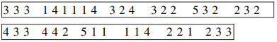
Example: Job set 5 is made up of five jobs with a total of thirteen operations. As a result, the solution vector comprises 13 parameters, which are shown below along with their jb-on, MC, and tool coding.
|
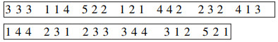
Following this, the solution vector for the starting population will be found.
|
Because the provided solutions for the initial population adhere to precedence restrictions, they are viable options.
Assessment: The MSN value of every vector in the first population is determined, and the vector in the initial population with the best MSN is chosen to form the basis for the succeeding generation.
If the input vector is, for instance,
|
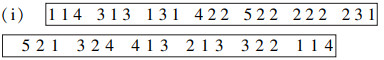
After assessing all of the vectors in the initial population, the best one (with the lowest MSN) is chosen. The best of the initial population is shown below.
|
make span=80
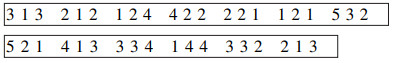
Below is a vector j, and j′ ≠ i is chosen at random.
|
In the mutualism phase, new solutions are generated and presented using Eqs. (14) and (15).
New solution(i):
|
New solution(j):
|
The previous solution will only be replaced by the new solution if the new solution offers a superior value; otherwise, the old solution will be used.
In the commensalism stage, a fresh solution is generated as per Eq. (16) and presented below.
Below is a randomly chosen vector k with the values k, 'k ≠ i' and 'k ≠ j'.
|
New solution(i):
|
The previous solution will only be replaced by the new solution if the new solution offers a superior value; otherwise, the previous solution will remain in place.
A vector l, 'l ≠ i', 'l ≠ j' and 'l ≠ k' is chosen at random to create a fresh solution for the parasitism phase, and it is depicted below.
|
New solution(i)
|
The fresh vector fitness value is compared to the fitness value of solution (i) and if it is higher, the vector i is replaced by fresh vector. This procedure is repeated until all candidates in the population have been eliminated, and then it is repeated until a specific number of generations have been finished; the optimal sequence up to this point is shown below.
|
Based on Venkat Rao's populace-built merging approach, the JAYA algorithm[55] is designed to solve a range of optimization problems, including constrained and unconstrained issues. The Jaya method generates P initial solutions at random while adhering to the process variables' upper and lower limits. Following that, Eq. (18) is used to stochastically update each variable of each solution. The best solution has the objective function's lowest value, whereas the worst solution has the objective function's highest value.
| $ \begin{aligned} y_{i, j}^{\prime} & =y_{i, j}+\operatorname{rand1} \times\left(y_{\text {best }, j}-\operatorname{abs}\left(y_{i, j}\right)\right)- \\ & \operatorname{rand2} \times\left(y_{\text {worst }, j}-\operatorname{abs}\left(y_{i, j}\right)\right) \end{aligned} $ | (18) |
where ybest, j and yworst, j correspond to the jth iteration's greatest and worst fitness values. yi, j' is the modified value of yi, j and abs(yi, j) is the absolute value of yi, j. rand2 and rand1 are numbers produced randomly in the range of [0, 1]. The term rand1×(ybest, j-abs(yi, j)) indicates the solution's propensity to go closer to the optimum solution, whereas the term-rand2×(yworst, j-abs(yi, j)) indicates the solution's inclination to shun the worst solution. If yi, j' yields a superior function value, it is acceptable. All of the acceptable function values at the conclusion of each iteration are kept and used as the input for the following iteration.
Algorithm
1.Set the size of population (IPZ), the number of design variables and criteria to fulfil, and the maximum number of iterations. (Max iter)
2.Analyze each candidate's fitness function value;
3.iter = 1;
4.While iter < Max_iter do
5.From the population, choose the best ybest and worst yworst candidates;
6.For i = 1 to IPZ do
7.Generate the updated solution.
8.Calculate the modified candidate's fitness function value.
9.If the fresh solution is superior than the old one, accept it.
10.End for
11.iter = iter + 1
12.End while.
3 Results and DiscussionsThe suggested approach is used for SMTTATWAM to minimize MSN. The control parameters of the algorithm are directly connected to the SOSA's efficiency. The algorithm's control parameters are the number of iterations and the population size. The algorithm was tested several times with various parameter values. As a result, in this study, the population number is set to 10 times the total operations in the job set, and the number of iterations is set to 125. Table 2 also shows the parameter values utilized in the SOSA. For MSN minimization, the MATLAB code for SMTTATWAM is performed 20 times on each problem outlined in Section 1.3.2. In Table 3, the best MSN from 20 runs is reported for each layout and job set for various scenarios, along with standard deviation (SDV) and mean. The Jaya algorithm, as reported in Venkat Rao[55], does not have any specific algorithmic parameters to be tuned. Therefore Jaya algorithm is applied for SMTTATWAM for MS minimization to show the efficacy of SOSA. Better values are obtained when the size of the population and the number of iterations are 10 times of operations and 70 times of job-set's operations, respectively.
| Table 2 SOSA control parameters |
| Table 3 Best MSN of SMAWAM for different job sets, layouts and cases along with SDV and mean |
For SOSA, the non zero SDV in Case 1 varies for LAOT 1 in the spectrum [0.0000, 2.0494], for LAOT 2 in the spectrum [0.0000, 1.6432], for LAOT3 in the spectrum [0.0000, 1.6234] and for LAOT 4 in the spectrum [0.0000, 2.3022], the non zero SDV in Case 2 varies for LAOT 1 in the spectrum [0.0000, 3.3122], for LAOT 2 in the spectrum [0.0000, 2.8284], for LAOT 3 in the spectrum [0.4472, 2.7386] and for Layout 4 in the spectrum [0.0000, 3.1937] and the non zero SDV in Case 3 varies for LAOT 4 in the range [0.0000, 1.4832].
For the Jaya algorithm in Case 1, the non-zero SDV varies in the band[1.4903, 3.1669] for LAYOUT 1, [1.0809, 3.4085] for LAYOUT 2, [1.4868, 3.4985] for LAYOUT 3, and [1.0915, 3.6201] for LAYOUT 4, in Case 2 it varies for LAYOUT 1 in the band[1.2312, 4.4544] for LAYOUT 2 in the band[1.8201, 4.4544], for LAYOUT 3 in the band[1.3870, 4.7780] and LAYOUT 4 in the band[1.9541, 4.7080] and in Case 3 for LAYOUT 4 it varies in the band[2.1734, 4.3175]. The coefficient of variation for non-zero SDV bands is from 0.00923 to 0.034275.
An intriguing discovery was made when they compared the size of the mean values to the standard deviation figures in Table 3, which showed that the typical deviation numbers were relatively low. In reality, for non-zero standard deviations, the coefficient of variation ranges between [0.002058, 0.025239]. Furthermore, for 24 of the 85 problems, the SDV is zero. Several solutions have the same MSN value when looking at the final solutions for these issues after 20 runs. It suggests many optima options out there, and the SOSA proposed can discover them.
When the best MSs, mean, and SDV obtained by SOSA are compared with the best MSNs, mean, and SDV obtained by the Jaya algorithm in Table 3, it is quite evident that SOSA outperforms the Jaya algorithm.
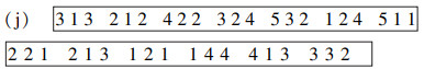
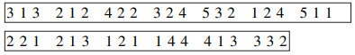
3.1 Gantt ChartThe Gantt chart depicts the viability of SOSA's best solution for minimal MSN for job set 5 LAOT 1 in Case 1. The optimal solution vector for Case 1, Layout 1, and job set 5 is shown below.
|
Table 4 is the table version of the solution mentioned above.
| Table 4 Optimal solution vector for job set 5, LAOT 1 of Case 1 |
Fig. 4 displays the Gantt chart for the solution vector mentioned above. A four-digit number is used to represent an operation. For example, in operation 4122, the job number is represented by the 1st digit '4', the 2nd digit '1' represents the jb-on, the 3rd digit '2' represents the needed MC, and the 4th digit '1' indicates the tool assigned to the jb-on. A Gantt chart displays the operations assigned to each MC and tool, along with the begin and finish times for each operation. The Gantt chart also displays the deadheaded trips, loaded trips, and TT wait times. Fig. 4 shows MCs M4, M2, M3, and M1, tools T4, T2, T3, and T1, and a tool transporter TT.

|
Fig.4 Gantt chart for the solution given in Table 4 |
LTT xxxx corresponds to operation xxxx's TT loaded trip. ETT xxxx corresponds to operation xxxx's TT empty trip. WPU XXXX stands for the TT waiting period for picking up the tool from the MC. WPL XXXX stands for the operation's TT waiting time before inserting the tool into the MC for operation xxxx.
Table 5 provides the best MSN of SMTTATWAM together with the best MSN of SMTTATWPM that was published in Sivarami Reddy et al.[30] and was achieved by SOSA, as well as the % decrease in MSN of SMTTATWAM over SMTTATWPM for a variety of job sets, layouts, and cases.
| Table 5 Best MSN of SMTTATWAM, Best MSN of SMTTATWPM obtained by SOSA and % reduction in MSN of SMTTATWAM over SMTTATWPM for various jobs, layouts and cases |
3.2 Convergence Characterstics
The SOSA convergence characteristics for Job set 4, Case 1, and layout 1 are displayed in Fig. 5.The optimal value of 79 was found at iteration number 83, and the average time spent on each iteration was 0.8661 s.

|
Fig.5 Convergence of SOSA for job set 4, LAOT 1 and Case 1 |
4 Case Study
This paper illustrates and evaluates the proposed scheduling strategy for a real world problem. The designated manufacturer serves southern India's automotive sector as a part supplier. The facility has five CNC milling MCs, one CNC lathe MC, CTM, and TT. Fig. 6 shows the layout of the facility. It receives component orders from various automotive businesses, develops a schedule based on the orders, manufactures the components, and promptly delivers them to the automotive businesses. The company produces casings, clamps, and slides. Initially, only primary MCs are scheduled for milling operations. This study takes into account the availability of alternative MCs for the same operation. A case study for SMTTATWAM is examined for MSN minimization, which takes into account alternative machines and tool transfer times between MCs on the shop floor. Table 6 displays a matrix of TT travel times.

|
Fig.6 Layout configuration for case study problem |
| Table 6 TT Travel time (Time in minutes) matrix for case study |
Casing, clamp, and slides each require eight, nine, and four operations, respectively. Table 7 contains information about such operations as well as alternative MCs. The processing time of an operation on any CNC milling MC is the same as they are identical. The operation of each component is represented by ONi, j, where i represents the component and j represents the operation. Processing time includes the time required to load and unload parts. Time for tool removal and placement is included in the tool transfer time. The main concern of this investigation is the selection of MCs and the assignment of tools to perform a operations of a job set and their sequences on the MC.
The job set has 9 components (3 indistinguishable casings, 3 indistinguishable clamps, and 3 indistinguishable slides) which have 63 operations. The details of job set are as follows.
component 1: casing-1; component 4 : casing-2;component 7 : casing-3; component 2: clamp-1; component 5 : clamp-2;component 8 : clamp-3; component 3: slide-1; component 6 : slide-2; component 9: slide-3.
| Table 7 Casing, clamp and slide operations details |
The following data is input for the code developed in MATLAB for SMTTATWAM with SOSA.
● TT's travel time matrix given in Table 6
● Number of parts in the job set and the data collected from Table 7 such as:
ⅰ)Each part's operations and parts' maximum operations in the job set.
ⅱ)Every part-operation necessitates the use of a machine (machine matrix).
ⅲ)Time required to complete each part-operation on the machine (process time matrix), and
ⅳ) Every part-operation necessitates the use of a tool (Tool matrix).
After evaluating the proposed SOSA and Jaya algorithms for SMTTATWAM, they are used to solve real case with 9 components (63 operations) on 6 MCs. Table 8 shows the decoded solution for the minimal. The numbers in brackets represent the start and end times of the operation and the tool specified for the operation. The results demonstrate the superiority of SOSA over the proposed Jaya, and the SOSA algorithm can identify near-optimal or ideal solutions to any large-scale problem. For this problem, the MSN calculated by SOSA and Jaya algorithm is 224 min and 239 min, respectively. Before implementing this technique, the firm uses SMTTATWPM employing primary MCs and produced components in 321 min. The reduction in MSN is 97 min.
| Table 8 SOSA and Jaya algorithm decoding solution in the form of MCs, and operations allocated to the MCs, as well as MSN |
5 Conclusions
This research presents a nonlinear MINLP model for MCs, TT, and tool joint shdng with alternative MCs, and one copy of each variety of tools in an MMFMS for minimum MSN. All of this is accomplished while taking into consideration tool switch times among MCs. This shdng problem entails assigning an appropriate MC and tool to each jb-ons, ordering and synchronizing those jb-ons on MCs, and enforcing constraints such as the number of copies of each tool variety and the TT for minimal MSN. Fig. 2 depicts the flow chart of an algorithm for computing MSN for a specified schedule. On the job sets specified in Section 1.3.2, the suggested method is tested. Table 3 shows that SOSA is resilient and capable of finding many optimal solutions to the problems. When best MSN values of both algorithms are compared, it is quite evident that SOSA outperforms the Jaya algorithm. Table 5 shows that using alternative MCs results in a considerable reduction in MSN. The decrease in MSN varies from 0.00 to 31.63. The manufacturer mentioned in the case study used to apply SMTTATWPM for manufacturing 9 components to supply to the automotive industry. The time it used to take to complete all the 9 components, i.e., MSN, is 321 min. When the manufacturer applied the proposed approach SMTTATWAM, the time it used to take to complete all 9 components is 224 min. There is a reduction of 97 min in MSN. A decrease in MSN indicates improvement in the utilization of resources. Integration of AGVs, robots, AS / RS, and tool change operations triggered by tool wear, the implementation of energy saving policies, with the integration of renewable energy sources, such as photovoltaic, wind, etc in the scheduling of manufacturing systems and also application of meta-heuristic optimization tools and its hybrid approaches to get optimal/near optimal solutions to address the problem can be a direction for future work.
Supplementary Materials Appendix-Ⅰ Notations and decision variables
Subscripts
j : job index
i, h, r: operations' sindices
k : index for a tool
g : MC index
J
job set meant for processing.
nj
job j's operations.
N
I
{1, 2, ……, N}, operations index set.
Ij
{Jj +1, Jj +2, ……, Jj+nj}, the collection of indices in "I" connected to job "j, " where "Jj" is the list of operations for jobs listed before job "j, " and J1=0.
ISi
I-{h; h≥i, i, h∈Ij} operations' index set with operations on the same job that follow operation i and not including operation i
IPh
I-{i; i≤h, i, h∈Ij} operations' index set with operations on the same job that precede operation h and not including operation h.
pgti(g)
processing duration for operation i on the MC, as denoted by g
pgti
processing time for operation i on a MC selected from a list of possibilities.
ctni
completion time for operation i on a chosen MC from the available options.
TL
a collection of several tool kinds to do the job-operations
TLCopy
copies of each variety of tool in a set.
Rk
indexes recorded in I coupled with TL using the tool type K.
indices set in I related with tool kind k in TL, ∀k∈TL
RTkj
Ij∩Rk the index set of operations in I shared by tool k and job j ∀k∈TL, ∀j∈J
u
first operation that makes use of tool K, u∈Rk, ∀k∈TL
v
i's preceding operation, i, v∈Rk, ∀k∈TL
L
number of TTs
aj
job j ready time
TMi(g)
ready time of MC indicated by g for operation i
TMi
selected MC ready time for operation i
AMi
{(x, y)/x: alternatemachine, y: Processing time for operation i on that machine}
the collection of alternative MCs and their processing times for operation i for ∀i∈I
tttdhi
Time taken for an empty flight between a MC doing operation h and a MC performing operation i.
tttli(g)
TT loaded flight 'i' travel time together with load and unload times for the MC indicated by g.
tttli
TT loaded trip 'i' travel time including load and unload times for the selected MC from available choices
CTTLi(g)
TT loaded flight i completion time for the MC indicated by g
CTTi
TT loaded trip i completion time for selected MC from available choices
Si
(max(TMi(g), CTTLi(g))+pgti(g))
mi
selected MC for operation i, ∀i∈I
MS
{ } collection of chosen MCs for operations related to I
Decision variables
| $ q_{\mathrm{rs}}=\left\{\begin{array}{l} 1, \text { if } \mathrm{ctn}_{\mathrm{r}} \text { is less than } \mathrm{ctn}_{\mathrm{s}}, \text { where } r \text { and } s \text { are operations of different jobs } \\ 0, \text { otherwise } \end{array}\right. $ |
| $\beta_{\mathrm{rs}}=\left\{\begin{array}{l} 0, \text { if } \mathrm{ctn}_{\mathrm{r}} \text { is less than } \mathrm{ctn}_{\mathrm{s}} \text {, where } r \text { and } s \text { are operations of different jobs, } r, s \in R_k \\ 1, \text { otherwise } \end{array}\right. $ |
| $ y_{\text {hi }}=\left\{\begin{array}{l} 1, \text { if TT is allocated for deadheading trip between trips } {}^{\prime}h^{\prime} \text { and } {}^{\prime}i^{\prime} \text { where the requested tool is accessible. } \\ 0, \text { otherwise } \end{array}\right. $ |
| $ y_{\text {oi }}=\left\{\begin{array}{l} 1, \text { if TT starts from CTM to accomplish trip } {}^{\prime}i^{\prime} \text { as its } 1 \text { st assignment } \\ 0, \text { otherwise } \end{array}\right. $ |
| $ y_{\mathrm{ho}}=\left\{\begin{array}{l} 1, \text { if TT returns the CTM after completing trip } {}^{\prime}h^{\prime} \text { as its last assignment } \\ 0, \text { otherwise } \end{array}\right. $ |
| $ \mathrm{ttt}_w=\left\{\begin{array}{l} \mathrm{tttd}_{\mathrm{o}, \mathrm{u}}, \text { if TT starts from CTM to accomplish trip } {}^{\prime}i^{\prime} \text { as its first accomplishment } \\ 0, \text { otherwise } \end{array}\right. $ |
Job set 1
Job set 2
Jb1: M/C1-T/L3 (8); M/C2-T/L4 (16); M/C4-T/L1 (12)
Jb1: M/C1-T/L3 (10); M/C4-T/L1 (18)
ALT1: M/C2-T/L3 (9) M/C3-T/L4 (14) M/C1-T/L1 (13)
ALT1: M/C3-T/L3 (12) M/C2-T/L1 (16)
ALT2: M/C3-T/L3 (9) M/C4-T/L4 (17) M/C2-T/L1 (10)
ALT2: M/C2-T/L3 (11) M/C3-T/L1 (17)
Jb2:M/C1-T/L2 (20); M/C3-T/L3 (10); M/C2-T/L1 (18)
Jb2:M/C2-T/L2 (10); M/C4-T/L4 (18)
ALT1: M/C3-T/L2 (18) M/C1-T/L3 (13) M/C4-T/L1 (17)
ALT1: M/C4-T/L2 (8); M/C1-T/L4 (20)
ALT2: M/C2-T/L2 (21) M/C4-T/L3 (8) M/C3-T/L1 (19)
ALT2: M/C3-T/L2(12); M/C2-T/L4 (16)
Jb3:M/C3-T/L1 (12); M/C4-T/L4 (8); M/C1-T/L2 (15)
Jb3:M/C1-T/L4 (10); M/C3-T/L2 (20)
ALT1: M/C4-T/L1 (11) M/C2-T/L4 (10) M/C3-T/L2 (14)
ALT1: M/C3-T/L4 (12); M/C2-T/L2 (18)
ALT2: M/C1-T/L1 (11) M/C3-T/L4 (7) M/C2-T/L2 (17)
ALT2: M/C2-T/L4 (8); M/C4-T/L2 (22)
Jb4:M/C4-T/L3 (14); M/C2-T/L4 (18)
Jb4:M/C2-T/L3 (10); M/C3-T/L1 (15); M/C4-T/L2 (12)
ALT1: M/C1-T/L3 (16) M/C3-T/L4 (16)
ALT1: M/C4-T/L3 (11) M/C1-T/L1 (17); M/C2-T/L2 (9)
ALT2: M/C3-T/L3 (16) M/C1-T/L4 (16)
ALT2: M/C1-T/L3 (13) M/C4-T/L1 (13); M/C3-T/L2 (11)
Jb5:M/C3-T/L2 (10); M/C1-T/L1 (15)
Jb5:M/C1-T/L4 (10); M/C2-T/L1 (15); M/C4-T/L3 (12)
ALT1: M/C2-T/L2 (9) M/C4-T/L1 (16)
ALT1: M/C4-T/L4 (12) M/C1-T/L1 (14); M/C3-T/L3 (11)
ALT2: M/C4-T/L2 (11) M/C3-T/L1 (14)
ALT2: M/C2-T/L4 (8) M/C3-T/L1 (14); M/C1-T/L3 (15)
Jb6:M/C1-T/L4 (10); M/C2-T/L2 (15); M/C3-T/L3 (12)
ALT1: M/C3-T/L4 (11) M/C4-T/L2 (13) M/C2-T/L3 (13)
ALT2: M/C2-T/L4 (12) M/C3-T/L2 (14) M/C4-T/L3 (11)
Job set 3
Job set 4
Jb1:M/C1-T/L4 (16); M/C3-T/L2 (15)
Jb1:M/C4-T/L2 (11); M/C1-T/L3 (10); M/C2-T/L1 (7)
ALT1: M/C3-T/L4 (14) M/C1-T/L2 (17)
ALT1: M/C3-T/L2(10) M/C2-T/L3(9) M/C4-T/L1(9)
ALT2: M/C2-T/L4 (15) M/C4-T/L2 (16)
ALT2: M/C2-T/L2(13) M/C4-T/L3(9) M/C3-T/L1(6)
Jb2:M/C2-T/L1 (18); M/C4-T/L3 (15)
Jb2:M/C3-T/L1 (12); M/C2-T/L2 (10); M/C4-T/L4 (8)
ALT1: M/C1-T/L1 (17) M/C3-T/L3 (16)
ALT1: M/C1-T/L1(10) M/C4-T/L2(11) M/C3-T/L4(9)
ALT2: M/C3-T/L1 (16) M/C2-T/L3 (17)
Jb3:M/C1-T/L3 (10); M/C2-T/L1 (10)
ALT1: M/C3-T/L3 (19) M/C4-T/L1 (11)
ALT2: M/C4-T/L3 (19) M/C1-T/L1 (11)
Jb4:M/C3-T/L3 (15); M/C4-T/L2 (10)
ALT1: M/C4-T/L3 (17) M/C2-T/L2 (8)
ALT2: M/C1-T/L3 (17) M/C3-T/L2 (8)
Jb5:M/C1-T/L4 (8); M/C2-T/L2 (10); M/C3-T/L3 (15);
M/C4-T/L4 (17)
ALT1: M/C3-T/L4(10) M/C4-T/L2(12) M/C2-T/L3(13)
M/C1-T/L4(15)
ALT2: M/C2-T/L4(9) M/C1-T/L2(8) M/C4-T/L3(13)
M/C3-T/L4(17)
Jb6:M/C2-T/L3 (10); M/C3-T/L1 (15); M/C4-T/L2 (8);
M/C1-T/L4 (15)
ALT1: M/C1-T/L3(8); M/C4-T/L1(14);M/C2-T/L2(10);M/C3-T/L4(16)
ALT2: M/C1-T/L3(9); M/C2-T/L1(16);M/C3-T/L2(9);
M/C4-T/L4(14)ALT2: M/C4-T/L1(11) M/C3-T/L2(9) M/C2-T/L4(10)
Jb3:M/C2-T/L2 (7); M/C3-T/L4 (10); M/C1-T/L3 (9);
M/C3-T/L2 (8)
ALT1: M/C4-T/L2(10) M/C2-T/L4(9) M/C3-T/L3(8)
M/C1-T/L2(7)
ALT2: M/C3-T/L2(9) M/C1-T/L4(11) M/C4-T/L3(7)
M/C2-T/L2(7)
Jb4:M/C2-T/L2 (7); M/C4-T/L3 (8);
M/C1-T/L1 (12);
M/C2-T/L2 (6)
ALT1: M/C3-T/L2(9) M/C2-T/L3(6) M/C4-T/L1(10)
M/C1-T/L2(8)
ALT2: M/C1-T/L2(8) M/C3-T/L3(9) M/C2-T/L1(9)
M/C4-T/L2(6)
Jb5:M/C1-T/L1 (9); M/C2-T/L3 (7); M/C4-T/L4 (8);
M/C2-T/L2 (10);M/C3-T/L3 (8)
ALT1: M/C3-T/L1(8) M/C4-T/L3(8) M/C3-T/L4(10)
M/C1-T/L2(9)M/C2-T/L3(7)
ALT2: M/C2-T/L1(8) M/C3-T/L3(8) M/C1-T/L4(9)
M/C3-T/L2(8)M/C4-T/L3(9)
Job set 5
Job set 6
Jb1:M/C1-T/L4 (6); M/C2-T/L1 (12); M/C4-T/L4 (9)
ALT1: M/C3-T/L4(7) M/C4-T/L1 (10) M/C2-T/L4 (10)
ALT2: M/C2-T/L4(7) M/C3-T/L1 (10) M/C1-T/L4 (10)
Jb2:M/C1-T/L2 (18); M/C3-T/L1 (6); M/C2-T/L3 (15)
ALT1: M/C3-T/L2 (16) M/C2-T/L1 (7) M/C1-T/L3 (16)
ALT2: M/C2-T/L2 (17) M/C4-T/L1 (8) M/C3-T/L3 (14)
Jb3:M/C3-T/L3 (9); M/C4-T/L4 (3); M/C1-T/L2 (12)
ALT1: M/C1-T/L3 (11) M/C3-T/L4 (4) M/C2-T/L2 (9)
ALT2: M/C4-T/L3 (10) M/C2-T/L4 (5) M/C3-T/L2 (11)
Jb4:M/C4-T/L2 (6); M/C2-T/L3 (15)
ALT1: M/C2-T/L2 (8) M/C3-T/L3 (13)
ALT2: M/C3-T/L2 (7) M/C1-T/L3 (14)
Jb5:M/C3-T/L2 (3); M/C1-T/L1 (9)
ALT1: M/C4-T/L2 (5) M/C2-T/L1 (7)
ALT2: M/C2-T/L2 (4) M/C4-T/L1 (8)Jb1:M/C1-T/L1 (9); M/C2-T/L2 (11); M/C4-T/L4 (7)
ALT1: M/C3-T/L1 (10) M/C1-T/L2 (9) M/C2-T/L4 (8)
ALT2: M/C4-T/L1 (11) M/C3-T/L2 (10) M/C1-T/L4(6)
Jb2:M/C1-T/L1 (19); M/C2-T/L2 (20);
M/C4-T/L4 (13)
ALT1: M/C4-T/L1 (20) M/C3-T/L2 (18) M/C2-T/L4 (14)
ALT2: M/C2-T/L1 (18) M/C3-T/L2 (22) M/C1-T/L4 (12)
Jb3:M/C2-T/L2 (14); M/C3-T/L3 (20); M/C4-T/L4 (9)
ALT1: M/C3-T/L2 (12) M/C4-T/L3 (21) M/C1-T/L4 (10)
ALT2: M/C4-T/L2 (15) M/C1-T/L3 (21) M/C2-T/L4 (7)
Jb4:M/C2-T/L2 (14); M/C3-T/L3 (20); M/C4-T/L4 (9)
ALT1: M/C4-T/L2 (13) M/C1-T/L3 (19) M/C3-T/L4 (11)
ALT2: M/C3-T/L2 (12) M/C4-T/L3 (19) M/C1-T/L4 (12)
Jb5:M/C1-T/L1 (11); M/C3-T/L3 (16); M/C4-T/L4 (8)
ALT1: M/C2-T/L1 (12) M/C1-T/L3 (14) M/C3-T/L4 (9)
ALT2: M/C3-T/L1 (12) M/C4-T/L3 (13) M/C2-T/L4 (10)
Jb6:M/C1-T/L1 (10); M/C3-T/L3 (12); M/C4-T/L4 (10)
ALT1: M/C3-T/L1(9) M/C4-T/L3 (11) M/C2-T/L4 (12)
ALT2: M/C2-T/L1 (9) M/C1-T/L3 (11) M/C3-T/L4 (12)
Job set 7
Job set 8
Jb1:M/C1-T/L1 (6); M/C4-T/L4 (6)
ALT1: M/C3-T/L1 (7) M/C2-T/L4 (5)
ALT2: M/C4-T/L1 (5) M/C3-T/L4 (7)
Jb2:M/C2-T/L2 (11); M/C4-T/L3 (9)
ALT1: M/C4-T/L2 (10) M/C3-T/L3 (10)
ALT2: M/C3-T/L2 (12) M/C1-T/L3 (8)
Jb3:M/C2-T/L2 (9); M/C4-T/L4 (7)
ALT1: M/C3-T/L2 (10) M/C1-T/L4 (6)
ALT2: M/C4-T/L2 (8) M/C3-T/L4 (8)
Jb4:M/C3-T/L3 (16); M/C4-T/L4 (7)
ALT1: M/C2-T/L3 (14) M/C3-T/L4 (9)
ALT2: M/C1-T/L3 (17) M/C2-T/L4 (6)
Jb5:M/C1-T/L1 (9); M/C3-T/L3 (18)
ALT1: M/C4-T/L1 (11) M/C2-T/L3(20)
ALT2: M/C2-T/L1 (10) M/C4-T/L3 (17)
Jb6:M/C2-T/L1 (13); M/C3-T/L2 (19); M/C4-T/L3 (6)
ALT1: M/C3-T/L1 (12) M/C4-T/L2 (18) M/C1-T/L3 (8)
ALT2: M/C1-T/L1 (14) M/C2-T/L2 (17) M/C3-T/L3 (7)
Jb7:M/C1-T/L3 (10); M/C2-T/L4 (9); M/C3-T/L1 (13)
ALT1: M/C3-T/L3 (11) M/C1-T/L4 (10) M/C2-T/L1 (11)
ALT2: M/C4-T/L3 (11) M/C3-T/L4 (10) M/C1-T/L1 (11)
Jb8:M/C1-T/L4 (11); M/C2-T/L2 (9); M/C4-T/L3 (8)
ALT1: M/C2-T/L4 (9) M/C3-T/L2 (10) M/C1-T/L3 (9)
ALT2: M/C4-T/L4 (10) M/C1-T/L2 (11) M/C3-T/L3 (7)Jb1:M/C2-T/L1 (12); M/C3-T/L2 (21); M/C4-T/L3 (11)
ALT1: M/C1-T/L1 (13) M/C4-T/L2 (19) M/C3-T/L3 (12)
ALT2: M/C3-T/L1 (14) M/C2-T/L2 (18) M/C1-T/L3 (12)
Jb2:M/C2-T/L4 (12); M/C3-T/L3 (21); M/C4-T/L2 (11)
ALT2: M/C1-T/L4 (13) M/C4-T/L3 (19) M/C3-T/L2 (12)
ALT1: M/C3-T/L4 (14) M/C2-T/L3 (20) M/C1(10)
ALT2: M/C1(13) M/C4(19) M/C3(12)
Jb3:M/C2-T/L2 (12); M/C3-T/L3 (21); M/C4-T/L4 (11)
ALT1: M/C4-T/L2 (13) M/C1-T/L3 (22) M/C3-T/L4 (9)
ALT2: M/C1-T/L2(10) M/C4-T/L3 (22) M/C2-T/L4 (12)
Jb4:M/C2-T/L1 (12); M/C3-T/L2 (21); M/C4-T/L3 (11)
ALT1: M/C3-T/L1 (11) M/C1-T/L2 (23) M/C2-T/L3 (10)
ALT2: M/C4-T/L1 (13) M/C2-T/L2 (22) M/C3-T/L3 (9)
Jb5:M/C1-T/L4 (10); M/C2-T/L1 (14); M/C3-T/L2 (18);
M/C4-T/L3 (9)
ALT1: M/C4-T/L4 (13) M/C3-T/L1 (13) M/C1-T/L2 (17)
M/C2-T/L3 (8)
ALT2: M/C3-T/L4 (11) M/C4-T/L1 (13) M/C2-T/L2 (16)
M/C1-T/L3 (11)
Jb6:M/C1-T/L2 (10); M/C2-T/L3 (14); M/C3-T/L (18);
M/C4-T/L1 (9)
ALT1: M/C2-T/L2 (12) M/C4-T/L3 (13) M/C1-T/L (16)
M/C3-T/L1 (10)
ALT2: M/C4-T/L2 (9) M/C3-T/L3 (15) M/C2-T/L (17)
M/C1-T/L1 (10)
Job set 9
Job set 10
Jb1:M/C3-T/L4 (9); M/C1-T/L2 (12); M/C2-T/L1 (9);
M/C4-T/L3 (6)
ALT1: M/C4(10) M/C3(9) M/C1(10)M/C2(7)
ALT2: M/C2(8) M/C4(15) M/C3(8)M/C1(5)
Jb2:M/C3-T/L4 (16); M/C2-T/L2 (11); M/C4-T/L3 (9)
ALT1: M/C1-T/L4 (14) M/C3-T/L2 (12) M/C2-T/L3 (10)
ALT2: M/C2-T/L4 (18) M/C4-T/L2 (10) M/C3-T/L3 (8)
Jb3:M/C1-T/L4 (21); M/C2-T/L2 (18); M/C4-T/L1 (7)
ALT1: M/C3-T/L4 (19) M/C4-T/L2 (19) M/C1-T/L1 (8)
ALT2: M/C4-T/L4 (22) M/C1-T/L2 (16) M/C2-T/L1 (8)
Jb4:M/C2-T/L4 (20); M/C3-T/L3 (22); M/C4-T/L2 (11)
ALT1: M/C4-T/L4 (21) M/C1-T/L3 (20) M/C3-T/L2 (12)
ALT2: M/C3-T/L4 (22) M/C2-T/L3 (21) M/C1-T/L2 (10)
Jb5:M/C3-T/L4 (14); M/C1-T/L2 (16); M/C2-T/L1 (13);
M/C4-T/L3 (9)
ALT1: M/C2-T/L4 (15) M/C4-T/L2 (13) M/C1-T/L1 (14)
M/C3-T/L3 (10)
ALT2: M/C1-T/L4 (16) M/C3-T/L2 (14)M/C4-T/L1 (11)
M/C2-T/L3 (11)Jb1:M/C1-T/L4 (11); M/C3-T/L3 (19); M/C2-T/L2 (16);
M/C4-T/L1 (13)
ALT1: M/C2-T/L4 (13) M/C4-T/L3 (17) M/C3-T/L2 (14)
M/C1-T/L1 (15)
ALT2: M/C4-T/L4 (13) M/C2-T/L3 (18) M/C1-T/L2 (14)
M/C3-T/L1 (14)
Jb2:M/C2-T/L3 (21); M/C3-T/L1 (16); M/C4-T/L2 (14)
ALT1: M/C3-T/L3 (19) M/C4-T/L1 (17) M/C1-T/L2 (15)
ALT2: M/C1-T/L3 (20) M/C4-T/L1 (18) M/C3-T/L2 (13)
Jb3:M/C3-T/L4 (8); M/C2-T/L2 (10); M/C1-T/L3 (14);
M/C4-T/L2 (9)
ALT1: M/C2-T/L4(10); M/C4-T/L2 (8); M/C3-T/L3 (16);
M/C1-T/L2 (7)
ALT2: M/C1-T/L4(10); M/C4-T/L2(8); M/C2-T/L3 (15);
M/C3-T/L2(8)
Jb4:M/C2-T/L3 (13); M/C3-T/L2 (20); M/C4-T/L4 (10)
ALT1: M/C1-T/L3 (15) M/C4-T/L2 (17) M/C3-T/L4 (11)
ALT2: M/C3-T/L3 (11) M/C1-T/L2 (20) M/C2-T/L4 (12)
Jb5:M/C1-T/L4 (9); M/C3-T/L3 (16); M/C4-T/L1 (18)
ALT1: M/C3-T/L4 (12) M/C4-T/L3 (14) M/C1-T/L1 (17)
ALT2: M/C4-T/L4 (10) M/C1-T/L3 (17) M/C2-T/L1 (16)
Jb6:M/C2-T/L4(19); M/C1-T/L3(21); M/C3-T/L1(11);
M/C4-T/L2 (15)
ALT1: M/C1-T/L4(16);
M/C3-T/L3(22); M/C4-T/L1(14);M/C2-T/L2 (14)
ALT2: M/C4-T/L4(17); M/C2-T/L3(19);
M/C1-T/L1(13);M/C3-T/L2 (17)
| [1] |
Agnetis Alessandro, Arianna Alfieri, Paolo Brandimarte, et al. Joint job/tool scheduling in a flexible manufacturing cell with No On-board tool magazine. Computer Integrated Manufacturing System, 1997, 10(1): 61-68. DOI:10.1016/S0951-5240(96)00023-7 (  0) 0) |
| [2] |
Saravanan M, Noorul Haq A. Evaluation of scatter-search approach for scheduling optimization of flexible manufacturing systems. The International Journal of Advanced Manufacturing Technology, 2008, 38: 978-986. DOI:10.1007/s00170-007-1134-5 ( 0) |
| [3] |
Chen F F, Adam E. The impact of flexible manufacturing systems on productivity and quality. IEEE Transactions on Engineering Management, 1991, 38(1): 33-45. DOI:10.1109/17.65758 ( 0) |
| [4] |
Jyothi D, Certificate Bonafide, Jyothi Divya, et al. Scheduling flexible manufacturing system using petri-nets and genetic algorithm. Project Report Indian Institute of Space Science and Technology, Thiruvananthapuram. 2013. https://www.semanticscholar.org/paper/SCHEDULING-FLEXIBLE-MANUFACTURING-SYSTEM-USING-AND-Jyothi-Certificate/e1bf3715e5a46f123bd8f19ef81ca1d2f8840df2
( 0) |
| [5] |
Shirazi Rabia, Frizelle G D M. Minimizing the number of tool switches on a flexible machine: An empirical study. International Journal of Production Research, 2001, 39(15): 3547-3560. DOI:10.1080/00207540110060888 ( 0) |
| [6] |
Tang C S, Denardo E V. Models arising from a flexible manufacturing machine, Part Ⅰ: Minimization of the number of tool switches. Operations Research, 1988, 36(5): 767-777. DOI:10.1287/opre.36.5.767 ( 0) |
| [7] |
Chandra P, Li S, Stan M. Jobs and tool sequencing in an automated manufacturing environment. International Journal of Production Research, 1993, 31(12): 2911-2925. DOI:10.1080/00207549308956907 ( 0) |
| [8] |
Song Chang-Yong, Hark Hwang, Yeong-Daekim. Heuristic algorithm for the tool movment policy in flexible manufacturing systems. Journal of Manufacturing Systems, 1995, 14(3): 160-168. DOI:10.1016/0278-6125(95)98884-9 ( 0) |
| [9] |
Roh H-K, Kim Y-D. Due-date based loading and scheduling methods for a flexible manufacturing system with an automatic tool transporter. International Journal of Production Research, 1997, 35(11): 2989-3004. DOI:10.1080/002075497194255 ( 0) |
| [10] |
Tsukada T K, Shin Kang G. Distributed tool sharing in flexible manufacturing systems. IEEE Transactions on Robotics and Automation, 1998, 14(3): 379-389. DOI:10.1109/70.678448 ( 0) |
| [11] |
Jun Hong-Bae, Kim Yeong-Dae, Suh Hyo-Won. Heuristics for a tool provisioning problem in a flexible manufacturing system with an automatic tool transporter. IEEE Transactions on Robotics and Automation, 1999, 15(3): 488-496. DOI:10.1109/70.768181 ( 0) |
| [12] |
Keung K W, Ip W H, Lee T C. A genetic algorithm approach to the multiple machine tool selection problem. Journal of Intelligent Manufacturing, 2001, 12: 331-342. DOI:10.1023/A:1011215416734 ( 0) |
| [13] |
Ecker K H, Gupta J N D. Scheduling tasks on a flexible manufacturing machine to minimize tool change delays. European Journal of Operational Research, 2005, 164: 627-638. DOI:10.1016/j.ejor.2003.12.025 ( 0) |
| [14] |
Prabaharan T, Nakkeeran P R, Jawahar N. Sequencing and scheduling of job and tool in flexible manufacturing cell. International Journal of Advanced Manufacturing Technology, 2006, 29: 729-745. DOI:10.1007/s00170-005-2567-3 ( 0) |
| [15] |
Fatma KilinÇ Karzan, Meral Azizoǧlu. The tool transporter movements problem in flexible manufacturing systems. International Journal of Poduction Research, 2008(11): 3059-3084. DOI:10.1080/00207540601070135 ( 0) |
| [16] |
Suresh Kumar N, Sridharan R. Simulation Modeling and Analysis of part and tool flow control decisions in a flexible manufacturing system. Robotics and Computer Integrated Manufacturing, 2009, 25(4-5): 829-838. DOI:10.1016/j.rcim.2008.12.004 ( 0) |
| [17] |
Udhayakumar P, Kumanan S. Sequencing and scheduling of job and tool in a flexible manufacturing system using ant colony optimization algorithm. The International Journal of Advanced Manufacturing Technology, 2010, 50: 1075-1084. DOI:10.1007/s00170-010-2583-9 ( 0) |
| [18] |
Udhayakumar P, Kumanan S. Some metaheuristic approaches for optimising tardiness of job and tool in a flexible manufacturing system. International Journal of Advanced Operations Management, 2012(3): 219-252. DOI:10.1504/IJAOM.2012.047683 ( 0) |
| [19] |
Aldrin Raj J, Ravindran D, Saravanan M, et al. Simultaneous scheduling of machines and tools in multimachine flexible manufacturing system using artificial immune system algorithm. International Journal of Computer Integrated Manufaturing, 2014, 27(5): 401-414. DOI:10.1080/0951192X.2013.834461 ( 0) |
| [20] |
Özpeynirci S. A heuristic approach based on time-indexed modelling for scheduling and tool loading in flexible manufacturing systems. The International Journal of Advanced Manufacturing Technology, 2015, 77: 1269-1274. DOI:10.1007/s00170-014-6564-2 ( 0) |
| [21] |
Costa A, Cappadonna F A, Fichera S. Minimizing the total completion time on a parallel machine system with tool changes. Computers & Industrial Engineering, 2016, 91: 290-301. DOI:10.1016/j.cie.2015.11.015 ( 0) |
| [22] |
Reddy N S, Ramamurthy D V, Rao K P, et al. A novel metaheuristic method for simultaneous scheduling of machines and tools in multi machine FMS. IET Digital Library International Conference on Recent Trends in Engineering, Science & Technology, 2016, 1-6. DOI:10.1049/cp.2016.1489 ( 0) |
| [23] |
Sivarami Reddy N, Ramamurthy D V, Prahlada Rao K, et al. Simultaneous scheduling of machines and tools in multi machine FMS using crow search algorithm. International Journal of Engineering Science and Technology, 2017, 9(9S): 66-73. ( 0) |
| [24] |
Chaithanya M, Siva N, Reddy S, et al. Sequencing and scheduling of jobs and tools in a flexible manufacturing system using Jaya algorithm. International Journal for Research in Applied Science & Engineering Technology, 2017, 5(XI): 2461-2469. DOI:10.22214/IJRASET.2017.11344 ( 0) |
| [25] |
Andreza Cristina Beezao, Jean-Francüois Cordeau, Gilbert Laporte, et al. Scheduling identical parallel machines with tooling constraints. European Journal of Operational Research, 2017, 257(3): 834-844. DOI:10.1016/j.ejor.2016.08.008 ( 0) |
| [26] |
Adil Baykasoǧlu, Fehmi Burcin Ozsoydan. Minimizing tool switching and indexing times with tool duplications in automatic machines. International Journal of Advanced Manufacturing Technology, 2017, 89: 1775-1789. DOI:10.1007/s00170-016-9194-z ( 0) |
| [27] |
Gustavo Silva Paiva, Marco Antonio M Carvalho. Improved heuristic algorithms for the job sequencing and tool switching problem. Computers and Operations Research, 2017, 88: 208-219. DOI:10.1016/j.cor.2017.07.013 ( 0) |
| [28] |
Burak Gökgür, Brahim Hnich, Selin Özpeynirci. Parallel machine scheduling with tool loading: a constraint programming approach. International Journal of Production Research, 2018, 56(16): 5541-5557. DOI:10.1080/00207543.2017.1421781 ( 0) |
| [29] |
Sivarami Reddy N, Ramamurthy D V, Prahlada Rao K. Simultaneous scheduling of machines and tools considering tool transfer times in multimachine FMS using CSA. International Conference on Intelligent Computing and Applications, Advances in Intelligent Systems and Computing, 2018, 632: 421-432. DOI:10.1007/978-981-10-5520-1_39 ( 0) |
| [30] |
Sivarami Reddy N, Ramamurthy D V, Prahlada Rao K. Simultaneous scheduling of jobs, machines and tools considering tool transfer times in multiALT2: M/C2-T/L2 (4) M/C4-T/L1 (8)machine FMS using new nature-inspired algorithms. Int. J. Intelligent Systems Technologies and Applications, 2018, 17(1/2): 70-88. DOI:10.1504/IJISTA.2018.091588 ( 0) |
| [31] |
Sivarami Reddy N, Ramamurthy D V, Prahlada Rao K, et al. Integrated scheduling of machines, AGVs and tools in multi-machine FMS using crow search algorithm. International Journal of Computer Integrated Manufacturing, 2019, 32(11): 1117-1133. DOI:10.1080/0951192X.2019.1686171 ( 0) |
| [32] |
Sivarami Reddy N, Ramamurthy D V, Prahlada Rao K, et al. Practical simultaneous scheduling of machines, AGVs, tool transporter and tools in a multi machine FMS using symbiotic organisms search algorithm. International Journal of Computer Integrated Manufacturing, 2021, 34(2): 153-174. DOI:10.1080/0951192X.2020.1858503 ( 0) |
| [33] |
Padma Lalitha Mareddy, Sivarami Reddy Narapureddy, Venkata Ramamurthy Dwivedula, et al. Simultaneous scheduling of machines, tool transporter and tools in a multi machine flexible manufacturing system without tool delay using crow search algorithm. Jordan Journal of Mechanical and Industrial Engineering, 2022, 16(3): 403-419. ( 0) |
| [34] |
Padma Lalitha Mareddy, Sivarami Reddy Narapureddy, Venkata Ramamurthy Dwivedula, et al. Optimum scheduling of machines, automated guided vehicles and tools without tool delay in a multi-machine flexible manufacturing system using symbiotic organisms search algorithm. Concurrency and Computation: Practice and Experience, 2022, 34(15): e6950. DOI:10.1002/cpe.6950 ( 0) |
| [35] |
Wilhelm W E, Shin Hyun-Myung. Effectiveness of alternative operations in a flexible manufacturing system. International Journal of Production Research, 1985, 23(1): 65-79. DOI:10.1080/00207548508904691 ( 0) |
| [36] |
Nasr Nabil, Elsayed E A. Job shop scheduling with alternative machines. International Journal of Production Research, 1990, 28(9): 1595-1609. DOI:10.1080/00207549008942818 ( 0) |
| [37] |
Ilkyeong Moon, Lee Jieom. Genetic Algorithm Application to the Job Shop Scheduling Problem with Alternative Routings. Pusan: Pusan National University, 2000.
( 0) |
| [38] |
Satish Kumar M V, Janardhana R, Rao C S P. Simultaneous scheduling of machines and vehicles in an FMS environment with alternative routing. The International Journal of Advanced Manufacturing Technology, 2011, 53: 339-351. DOI:10.1007/s00170-010-2820-2 ( 0) |
| [39] |
Sivarami Reddy N, Padma Lalitha M, Pandey S P, et al. Simultaneous scheduling of machines and tools in a multimachine FMS with alternative routing using symbiotic organisms search algorithm. Journal of Engineering Research, 2022, 10(3A): 274-297. DOI:10.36909/jer.10653 ( 0) |
| [40] |
Sivarami Reddy N, Padma Lalitha M, Ramamurthy D V, et al. Simultaneous Scheduling of machines and tools in a multi-machine FMS with alternate machines using crow search algorithm. Journal of Advanced Manufacturing Systems, 2022, 21(1): 1-24. DOI:10.1142/S0219686722500305 ( 0) |
| [41] |
Lenstra J K, Rinnooy Kan A H G. Computational complexity of discrete optimization problems. Ann. Discrete Math., 1979, 4(121): 140. DOI:10.1016/S0167-5060(08)70821-5 ( 0) |
| [42] |
Lenstra J K, Rinnooy Kan A H G. Complexity of vehicle routing and scheduling problems. Networks, 1981, 11(2): 221-227. DOI:10.1002/net.3230110211 ( 0) |
| [43] |
Al-Refaie A. Optimal scheduling and sequencing of operating room under emergency cases. Jordan Journal of Mechanical & Industrial Engineering, 2017, 11(1): 21-26. ( 0) |
| [44] |
Abbas Al-Refaie, Hala Abedalqader. Optimal quay crane assignment and scheduling in port's container terminals. Jordan Journal of Mechanical and Industrial Engineering, 2021, 15(2): 153-167. ( 0) |
| [45] |
Carlucci D, Paolo Renna, Sergio Materi. A job-shop scheduling decision-making model for sustainable production planning with power constraint. IEEE Transactions on Engineering Management, 2021, 99: 1-10. ( 0) |
| [46] |
Renna P, Sergio Materi. A literature review of energy efficiency and sustainability in manufacturing systems. Appl. Sci., 2021, 11(16): 7366. DOI:10.3390/app11167366 ( 0) |
| [47] |
Fernandes J M R C, Homayouni S M, Fontes D B M M. Energy-efficient scheduling in job shop manufacturing systems: a Literature review. Sustainability, 2022, 14: 6264. DOI:10.3390/su14106264 ( 0) |
| [48] |
Cheng Min-Yuan, Doddy Prayogo. Symbiotic organisms search: a new metaheurstic optimization algorithm. Computers and Structures Structures, 2014, 139: 98-112. DOI:10.1016/j.compstruc.2014.03.007 ( 0) |
| [49] |
Wu Haizhou, Zhou Yongquan, Luo Qifang, et al. Training feedforward neural networks using symbiotic organisms search algorithm. Computational Intelligence and Neuroscience, 2016, 2016: Article ID 9063065. DOI: 10.1155/2016/9063065.
( 0) |
| [50] |
Ghanshyam G Tejani, Vimal J Savsanin, Vivek K Patel. Adaptive symbiotic organisms search (SOS) algorithm for structural design optimization. Journal of Computational Design and Engineering, 2016, 3(3): 226-249. DOI:10.1016/j.jcde.2016.02.003 ( 0) |
| [51] |
Reddy Kommuri S, Sivarami Reddy S. Simultaneous scheduling of machines and AGVS in FMS by using Symbiotic Organisms Search (SOS) Algorithm. International Journal for Research in Applied Science & Engineering Technology, 2017, 5(XI): 1780-1790. DOI:10.22214/ijraset.2017.11258 ( 0) |
| [52] |
Sonmez Yusuf, Tolga Kahraman H, Kenan Dosoglu M, et al. Symbiotic organisms search algorithm for dynamic economic dispatch with valve-point effects. Journal of Experimental & Theoretical Artificial Intelligence, 2017, 29(3): 495-515. DOI:10.1080/0952813X.2016.1198935 ( 0) |
| [53] |
Reza Safipour, Mahmoud Oukati Sadegh. Optimal planning of energy storage systems using symbiotic organisms search algorithm. International Journal of Industrial Electronics, Control and Optimization, 2018, 1(1): 19-26. ( 0) |
| [54] |
Bilge Ümit, Gündüz Ulusoy. A time window approach to simultaneous scheduling of machines and material handling system in FMS. Operations Research, 1995, 43: 1058-1070. DOI:10.1287/opre.43.6.1058 ( 0) |
| [55] |
Venkata Rao R. Jaya: A simple and new optimization algorithm for solving constrained and unconstrained optimization problems. International Journal of Industrial Engineering Computations, 2016, 7: 19-34. ( 0) |