We introduce the notion of inertial entropy, a characteristic of partitions of finite metric spaces. This type of entropy and metrics associated with it are used to investigate the quality of hierarchical clusterings of objects that occur in a metric space.
Inertial entropy belongs to a broader family of numerical characteristics of partitions of finite sets[1]. It can be used to evaluate how tight objects are grouped around the cluster centers and the similarity of two partitions of a set of objects. In turn, this similarity allows us to evaluate how close a partition produced by a clustering algorithm is to a reference partition determined by the labels of the objects.
Partitions that define clusterings may be obtained via a diversity of clustering algorithms. In particular, hierarchical clustering algorithms construct chains of partitions of the set of objects referred usually as a dendrograms. The blocks of the initial dendrogram partition of the set of objects S are singletons. Starting from a given partition of S, a new partition is constructed by fusing a pair of blocks of the previous partition in the chain. The blocks to be fused are selected according to a criterion specific to the clustering method. A variety of methods[2] have been developed for constructing such clusterings (single-link, complete-link, Ward clusterings, group-average, centroid clusterings, etc.). Each of these methods facilitates favors finding certain types of clusters (elongated clusters in the case of single-link, globular clusters in the case of complete-link, etc.)
A distinct line of research is the consideration of generalization of entropy in the context of fuzzy sets[3-4]. Also, an interesting line of research is the use of entropy in the study of the singular values of tensors related to hypergraphs[5].
We define entropy using partitions rather than probability distributions. This is justified by the fact that sets of partitions have a rich algebraic structure, while probability distributions are limited to reflecting the sizes of the blocks of partitions. Indeed, as we see next, the set of partitions of a set can be naturally equipped with a partial order such that the set of partitions of a finite set is a semimodular lattice with respect to this partial order or a geometric lattice (see Ref.[6]). Partitions are also more expressive than probability distributions because they capture the relationships between set elements and the partition blocks where they are located.
The exploration of entropy axiomatization has a long tradition in information theory. Relevant work includes the results of Khinchin[7], Faddeev[8], Ingarden and Urbanik[9]. Daróczy[10], Havrda and Charvat[11], and Tsallis and Furuichi[12-13] who introduced generalizations of entropy that are suitable for partitions of unstructured spaces. The entropy proposed here deals with partitions of objects placed in metric spaces and makes use of concepts related to the metric space structure such as distance, centroid, etc.
In Section 1, we introduce partitions and discuss properties of the partial ordered set of partitions. In Section 2, we introduce an axiomatization of generalized entropy for partitions which yields, as the special case the Shannon entropy. Since the entropy proposed in this note applies to sets of objects located in metric spaces, we introduce the inertia and the notion of centroid of a set and establish the monotonicity of the sum of square errors in Section 3. The inertial entropy and its axiomatization are presented in Section 4. Note that the proposed axiomatization is an adaptation of the general axiomatization to the sets of objects located in metric spaces where the notions of inertia of a set of objects and sum of square errors are applicable. Conditional inertial entropies and metrics generated by these entropies are studied in Section 5. Section 6 presents an application of the metric space of partitions defined by the distance generated by the inertial entropy to clustering technique validation of labeled data. Section 7 presents ideas for future work.
1 Partitions of Finite SetsWe introduce some basic facts that concern partitions. Formally, a partition of a set S is a collection of non-empty subsets of S referred to as blocks,
Set partitions are fundamental for the study of clusterings because a non-overlapping set clustering can be viewed as a partition whose blocks are the clusters. Thus, we will use the terms "partition block" and "cluster" interchangeably.
A partial order "
If
If S, T are two non-empty, disjoint sets and
| $ \sigma+\tau=\left\{B_{1}, B_{2}, \cdots, B_{m}, C_{1}, C_{2}, \cdots, C_{n}\right\} $ |
Furthermore, if S, T, U are non-empty disjoint sets,
| $\sigma+(\tau+\nu)=(\sigma+\tau)+\nu $ |
a property referred to as the associativity of partition addition. If S and T are non-empty disjoint sets, then
| $ \alpha_{S}+\alpha_{T}=\alpha_{S \cup T} $ |
If
| $ \sigma=\omega_{B 1}+\omega_{B 2}+\cdots+\omega_{B m} $ |
If the set S consists of a single element, S={s}, then
In the previous work[1], we proposed an axiomatization of partition entropy for partitions of finite sets that takes into account the number of elements of the blocks of the partition. The sizes of partition blocks define a probability distribution and this leads to the idea of axiomatizing the entropy of partitions. The proposed system of axioms for partition entropy
(P1) If
(P2) If A and B are two finite sets such that
(P3) For every disjoint sets A, B and partition
| $ \begin{aligned} & H_{\beta}(\pi+\sigma)=\left(\frac{|A|}{|A|+|B|}\right)^{\beta} H_{\beta}(\pi)+ \\ & \quad\left(\frac{|B|}{|A|+|B|}\right)^{\beta} H_{\beta}(\sigma)+H_{\beta}(\{A, B\}) \end{aligned} $ |
(P4) If
| $H_{\beta}(\pi \times \sigma)=\varPhi\left(H_{\beta}(\pi), H_{\beta}(\sigma)\right) $ |
where
It was shown in Ref.[1] that a function
| $H_{\beta}=\frac{1}{2^{1-\beta}-1}\left(1-\sum\limits_{i=1}^{m}\left(\frac{\left|B_{i}\right|}{|S|}\right)^{\beta}\right) $ |
When
| $ \lim _{\beta \rightarrow 1, \beta>1} H_{\beta}(\pi)=-\sum\limits_{i=1}^{m} \frac{\left|B_{i}\right|}{|S|} \log _{2} \frac{\left|B_{i}\right|}{|S|} $ |
which corresponds to Shannon entropy.
The
When the set S is a subset of a metric space, it becomes possible to define an entropy-like measure that is defined by the scattering of the elements of blocks around the centroids of these blocks, which supplements the description of partitions. This new measure defined in Section 4, which we refer to as the inertial entropy takes advantage of the metric structure that exists for the set of objects.
3 Inertia of a Set of PointsThe notion of inertia of a non-empty finite subset S of
| $ I_{z}=\sum\limits_{x \in S}\|\boldsymbol{x}-\boldsymbol{z}\|_{2}^{2} $ |
If
The centroid of a non-empty finite set of vectors
| $ c_{s}=\frac{1}{|S|} \sum\limits_{i=1}^{m} \boldsymbol{x}_{\boldsymbol{i}} $ |
Huygens' Inertia Theorem (see Ref.[2]) stipulates that
| $ I_{z}(S)-I_{c S}(S)=|S|\left\|\boldsymbol{c}_{S}-\boldsymbol{z}\right\|_{2}^{2} $ |
for every
It is immediate that if
| $\begin{equation*} \operatorname{sse}(S)=\sum\limits_{\boldsymbol{x} \in S}\|\boldsymbol{x}\|^{2}-|S|\left\|\boldsymbol{c}_{S}\right\|^{2} \end{equation*} $ | (1) |
Furthermore, the set S is a singleton then sse(S)=0.
Clustering sets of vectors in
Theorem 1 Let W be a subset of S and let
| $ \begin{aligned} & \operatorname{sse}(W)=\operatorname{sse}(U)+\operatorname{sse}(V)+\frac{|U||V|}{|W|} . \\ & \quad\left\|\boldsymbol{c}_{U}-\boldsymbol{c}_{V}\right\|^{2} \end{aligned} $ |
Proof By applying the definition of the sum of square errors we have:
| $ \begin{aligned} & \operatorname{sse}(W)-\operatorname{sse}(U)-\operatorname{sse}(V)=\sum\left\{\left\|\boldsymbol{x}-\boldsymbol{c}_{W}\right\|^{2} \mid\right. \\ & \quad \boldsymbol{x} \in U \cup V\}-\sum\left\{\left\|\boldsymbol{x}-\boldsymbol{c}_{U}\right\|^{2} \mid \boldsymbol{x} \in U\right\}- \\ & \quad \sum\left\{\left\|\boldsymbol{x}-\boldsymbol{c}_{V}\right\|^{2} \mid \boldsymbol{x} \in V\right\} \end{aligned} $ |
The centroid of W is given by:
| $ \boldsymbol{c}_{W}=\frac{1}{|W|} \sum\{\boldsymbol{x} \mid \boldsymbol{x} \in W\}=\frac{|U|}{|W|} \boldsymbol{c}_{U}+\frac{|V|}{|W|} \boldsymbol{c}_{V} $ |
This allows us to evaluate the variation of the sum of squared errors:
| $ \begin{aligned} & \operatorname{sse}(W)-\operatorname{sse}(U)-\operatorname{sse}(V)=\sum\left\{\left\|\boldsymbol{x}-\boldsymbol{c}_{W}\right\|^{2} \mid\right. \\ & \quad \boldsymbol{x} \in U \cup V\}-\sum\left\{\left\|\boldsymbol{x}-\boldsymbol{c}_{U}\right\|^{2} \mid \boldsymbol{x} \in U\right\}- \\ & \sum\left\{\left\|\boldsymbol{x}-\boldsymbol{c}_{V}\right\|^{2} \mid \boldsymbol{x} \in V\right\}=\sum\left\{\left\|\boldsymbol{x}-\boldsymbol{c}_{W}\right\|^{2}-\right. \\ & \left.\left\|\boldsymbol{x}-\boldsymbol{c}_{U}\right\|^{2} \mid \boldsymbol{x} \in U\right\}+\sum\left\{\left\|\boldsymbol{x}-\boldsymbol{c}_{W}\right\|^{2}-\right. \\ & \left.\left\|\boldsymbol{x}-\boldsymbol{c}_{V}\right\|^{2} \mid \boldsymbol{x} \in V\right\} \end{aligned} $ |
Observe that:
| $ \begin{aligned} & \sum\left\{\left\|\boldsymbol{x}-\boldsymbol{c}_{W}\right\|^{2}-\left\|\boldsymbol{x}-\boldsymbol{c}_{U}\right\|^{2} \mid \boldsymbol{x} \in U\right\}= \\ & \sum\limits_{\boldsymbol{x} \in U}\left(\left(\boldsymbol{x}-\boldsymbol{c}_{W}\right)^{\prime}\left(\boldsymbol{x}-\boldsymbol{c}_{W}\right)-\left(\boldsymbol{x}-\boldsymbol{c}_{U}\right)^{\prime}\left(\boldsymbol{x}-\boldsymbol{c}_{U}\right)\right)= \\ & |U|\left(\boldsymbol{c}_{W}^{\prime} \boldsymbol{c}_{W}-\boldsymbol{c}_{U}^{\prime} \boldsymbol{c}_{U}\right)+2\left(\boldsymbol{c}_{U}^{\prime}-\boldsymbol{c}_{W}^{\prime}\right) \sum\limits_{x \in U} \boldsymbol{x}= \\ & |U|\left(\boldsymbol{c}_{W}^{\prime} \boldsymbol{c}_{W}-\boldsymbol{c}_{U}^{\prime} \boldsymbol{c}_{U}\right)+2|U|\left(\boldsymbol{c}_{U}^{\prime}-\boldsymbol{c}^{\prime}{ }_{W}\right) \boldsymbol{c}_{U}= \\ & |U|\left(\left\|\boldsymbol{c}_{W}\right\|^{2}-\left\|\boldsymbol{c}_{U}\right\|^{2}+2\left\|\boldsymbol{c}_{U}\right\|^{2}-2 \boldsymbol{c}^{\prime}{ }_{\boldsymbol{W}} \boldsymbol{c}_{U}\right)= \\ & |U|\left(\left\|\boldsymbol{c}_{W}\right\|^{2}+\left\|\boldsymbol{c}_{U}\right\|^{2}-2 \boldsymbol{c}_{W}^{\prime} \boldsymbol{c}_{U}\right)=|U|\left\|\boldsymbol{c}_{W}-\boldsymbol{c}_{U}\right\|^{2} \end{aligned} $ |
Using the equality
| $ \begin{equation*} \boldsymbol{c}_{W}-\boldsymbol{c}_{U}=\frac{|U|}{|W|} \boldsymbol{c}_{U}+\frac{|V|}{|W|} \boldsymbol{c}_{V}-\boldsymbol{c}_{U}= \\ \frac{|V|}{|W|}\left(\boldsymbol{c}_{V}-\boldsymbol{c}_{U}\right) \end{equation*} $ | (2) |
The following equation is obtained
| $ \begin{aligned} \sum\{ & \left.\left\|\boldsymbol{x}-\boldsymbol{c}_{W}\right\|^{2}-\left\|\boldsymbol{x}-\boldsymbol{c}_{U}\right\|^{2} \mid \boldsymbol{x} \in U\right\}= \\ & \frac{|U||V|^{2}}{|W|^{2}}\left\|\boldsymbol{c}_{V}-\boldsymbol{c}_{U}\right\|^{2} \end{aligned} $ |
In a similar manner, we have:
| $ \left\{\boldsymbol{x}-\boldsymbol{c}_{W}\left\|^{2}-\right\| \boldsymbol{x}-\boldsymbol{c}_{V} \|^{2} \mid \boldsymbol{x} \in V\right\}= \\ \frac{|U|^{2}|V|}{|W|^{2}} \cdot\left\|\boldsymbol{c}_{V}-\boldsymbol{c}_{U}\right\|^{2} $ |
so,
| $ \begin{align*} \operatorname{sse}(W)-\operatorname{sse}(U)-\operatorname{sse}(V)=\frac{|U||V|}{|W|} . \\ \quad\left\|\boldsymbol{c}_{V}-\boldsymbol{c}_{U}\right\|^{2} \end{align*} $ | (3) |
which is the needed equality.
Corollary 1 If U, W are two subsets of
Proof Since
If
| $\begin{equation*} \operatorname{sse}(\pi)=\sum\limits_{i=1}^{m} \operatorname{sse}\left(B_{i}\right) \end{equation*} $ | (4) |
Note that
The sum of the square errors of a partition plays an important role in analyzing properties of various clustering algorithms. One example is the proof of convergence of the k-means algorithm, where the sum of the square errors of the current clustering is decreasing for the chain of partitions obtained by successive object reassignments.
4 Inertial Entropy and Its AxiomatizationLet
·Initial values axiom: For every set S, we have
·Addition axiom: If S and T are finite disjoint sets,
| $H(\pi+\sigma)=\frac{\operatorname{sse}(S)}{\operatorname{sse}(S \cup T)} H(\pi)+\frac{\operatorname{sse}(T)}{\operatorname{sse}(S \cup T)} .\\ H(\sigma)+H(S, T) $ |
Note the similarity between the addition axiom for inertial entropy and the axiom P3 for partition entropy.
Lemma 1 Let U, V be two disjoint, finite, and non-empty subsets of
| $ H(\boldsymbol{\pi})=H\left(\pi^{\prime}\right)+\frac{\operatorname{sse}(V)}{\operatorname{sse}(U \cup V)} $ |
Proof By the Addition Axiom, we have:
| $ \begin{aligned} & H\left(\sigma+\alpha_{V}\right)=\frac{\operatorname{sse}(U)}{\operatorname{sse}(U \cup V)} H(\sigma)+\frac{\operatorname{sse}(V)}{\operatorname{sse}(U \cup V)}+ \\ & H(\{U, V\}) \end{aligned} $ |
and
| $ \begin{aligned} & H\left(\sigma+\omega_{V}\right)=\frac{\operatorname{sse}(U)}{\operatorname{sse}(U \cup V)} H(\sigma)+\frac{\operatorname{sse}(V)}{\operatorname{sse}(U \cup V)} . \\ & H\left(\omega_{V}\right)+H(\{U, V\})=\frac{\operatorname{sse}(U)}{\operatorname{sse}(U \cup V)} H(\sigma)+ \\ & H(\{U, V\}) \end{aligned} $ |
which implies
| $H(\pi)=H\left(\pi^{\prime}\right)+\frac{\operatorname{sse}(V)}{\operatorname{sse}(U \cup V)} $ |
because
The next theorem shows that the inertial entropy of a partition is a linear function of the sum of the square errors of the blocks of the partition.
Theorem 2 If
| $ H(\boldsymbol{\pi})=1-\frac{1}{\operatorname{sse}(S)} \sum\limits_{i=1}^{m} \operatorname{sse}\left(B_{i}\right)=1-\frac{\operatorname{sse}(\pi)}{\operatorname{sse}\left(\omega_{S}\right)} $ |
Proof Let
| $ \pi=\omega_{B_{1}}+\omega_{B_{2}}+\cdots+\omega_{B_{m}} $ |
Starting from
| $ \begin{gathered} \pi_{0}=\omega_{B_{1}}+\omega_{B_{2}}+\cdots+\omega_{B_{m}}=\pi \\ \pi_{1}=\alpha_{B_{1}}+\omega_{B_{2}}+\cdots+\omega_{B_{m}} \\ \pi_{2}=\alpha_{B_{1}}+\alpha_{B_{2}}+\cdots+\omega_{B_{m}} \\ \vdots \\ \pi_{m}=\alpha_{B_{1}}+\alpha_{B_{2}}+\cdots+\alpha_{B_{m}}=\alpha_{S} \end{gathered} $ |
Let
| $ \sigma_{i}=\alpha_{B_{1}}+\cdots+\alpha_{B_{i}}+\omega_{B_{i+2}}+\cdots+\omega_{B_{m}} \in \operatorname{PART}\left(S-B_{i+1}\right) $ |
Then, we have
| $ H\left(\pi_{i+1}\right)=H\left(\pi_{i}\right)+\frac{\operatorname{sse}\left(B_{i+1}\right)}{\operatorname{sse}(S)} $ |
Thus, we have
| $ \begin{gathered} H\left(\pi_{1}\right)=H\left(\pi_{0}\right)+\frac{\operatorname{sse}\left(B_{1}\right)}{\operatorname{sse}(S)} \\ H\left(\pi_{2}\right)=H\left(\pi_{1}\right)+\frac{\operatorname{sse}\left(B_{2}\right)}{\operatorname{sse}(S)} \\ \vdots \\ H\left(\pi_{m}\right)=H\left(\pi_{m-1}\right)+\frac{\operatorname{sse}\left(B_{m}\right)}{\operatorname{sse}(S)} \end{gathered} $ |
which yields
| $H(\boldsymbol{\pi})=1-\frac{1}{\operatorname{sse}(S)} \sum\limits_{i=1}^{m} \operatorname{sse}\left(B_{i}\right) $ |
An equivalent expression of the inertial entropy of a partition
| $ \begin{equation*} H(\boldsymbol{\pi})=\frac{\sum\limits_{i=1}^{n}\left|B_{i}\right|\left\|\boldsymbol{c}_{i}\right\|^{2}-|S|\|\boldsymbol{c}\|^{2}}{\sum\limits_{x \in S}\|\boldsymbol{x}\|^{2}-|S|\|\boldsymbol{x}\|^{2}} \end{equation*} $ | (5) |
where
Note that
Theorem 3 Let
| $ \begin{aligned} & H(\sigma)=H(\pi)-\frac{1}{\operatorname{sse}(S)} \frac{\left|B_{m-1}\right| \cdot\left|B_{m}\right|}{\left|B_{m-1}\right|+\left|B_{m}\right|} \| \boldsymbol{c}_{m-1}- \\ & \boldsymbol{c}_{m} \|^{2} \end{aligned} $ |
Proof By Theorem 1, we have:
| $ \begin{aligned} H(\sigma)= & 1-\frac{1}{\operatorname{sse}(S)}\left(\sum\limits_{i=1}^{m-2} \operatorname{sse}\left(B_{i}\right)+\operatorname{sse}\left(B_{m-1} \cup B_{m}\right)\right)= \\ & 1-\frac{1}{\operatorname{sse}(S)}\left(\sum\limits_{i=1}^{m-2} \operatorname{sse}\left(B_{i}\right)+\operatorname{sse}\left(B_{m-1}\right)+\operatorname{sse}\left(B_{m}\right)+\right. \\ & \left.\frac{\left|B_{m-1}\right| \cdot\left|B_{m}\right|}{\left|B_{m-1}\right|+\left|B_{m}\right|}\left\|\boldsymbol{c}_{m-1}-\boldsymbol{c}_{m}\right\|^{2}\right)=H(\boldsymbol{\pi})-\frac{1}{\operatorname{sse}(S)} \cdot \end{aligned} $ |
| $\frac{\left|B_{m-1}\right| \cdot\left|B_{m}\right|}{\left|B_{m-1}\right|+\left|B_{m}\right|}\left\|\boldsymbol{c}_{m-1}-\boldsymbol{c}_{m}\right\|^{2} $ |
Corollary 2 The inertial entropy is dually monotonic. In other words, if
Proof This is an immediate consequence of Theorem 3.
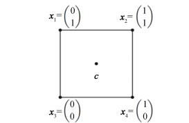
Example 1 Consider the set
| $ \boldsymbol{x}_{1}=\binom{0}{1}, \boldsymbol{x}_{2}=\binom{1}{1}, \boldsymbol{x}_{3}=\binom{0}{0}, \boldsymbol{x}_{4}=\binom{1}{0} $ |
|
Fig.1
Set |
And the partition
The centroid of
| $ \begin{gathered} \operatorname{sse}(S)=4\left(\frac{\sqrt{2}}{2}\right)^{2}=2 \\ \operatorname{sse}\left(\left\{\boldsymbol{x}_{1}, \boldsymbol{x}_{4}\right\}\right)=\left\|\boldsymbol{x}_{1}-\boldsymbol{c}\right\|^{2}+\left\|\boldsymbol{x}_{4}-\boldsymbol{c}\right\|^{2}=1 \\ \operatorname{sse}\left(\left\{\boldsymbol{x}_{2}, \boldsymbol{x}_{3}\right\}\right)=\left\|\boldsymbol{x}_{2}-\boldsymbol{c}\right\|^{2}+\left\|\boldsymbol{x}_{3}-\boldsymbol{c}\right\|^{2}=1 \end{gathered} $ |
hence
| $ \begin{gathered} H(\pi)=1-\frac{1}{\operatorname{sse}(S)}\left(\operatorname{sse}\left(\left\{\boldsymbol{x}_{1}, \boldsymbol{x}_{4}\right\}\right)+\operatorname{sse}\left(\left\{\boldsymbol{x}_{2}, \right.\right.\right. \\ \left.\left.\left.\boldsymbol{x}_{3}\right\}\right)\right)=1-\frac{1}{2}(1+1)=0 \end{gathered} $ |
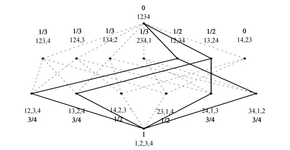
In Fig. 2, the inertial entropies of the partitions of the set S are shown in bold letters.
|
Fig.2
The annotated Hasse diagram of ( |
Theorem 3 implies that the decrease in inertial entropy that results by fusing two blocks of a partition is determined by the harmonic average of the size of the fused blocks and by the distance between the centroids of these blocks.
The choice of a particular hierarchical clustering method has an obvious impact on the variation of entropy. In each of the methods discussed below the pair of clusters (U, V) to be fused is selected such that the corresponding cluster dissimilarity is minimized.
Table 1 contains the cluster dissimilarity that is minimized when two clusters U and V are fused in some of the most popular hierarchical clustering methods.
| Table 1 Dissimilarities used in clutering methods |
This allows us to characterize sequences of partitions that are produced by Ward clusterings[14-15].
Theorem 4 Let S be a finite subset of
Proof Let
| $H\left(\pi_{i}\right)-H\left(\pi_{i+1}\right)=\frac{1}{\operatorname{sse}(S)} \operatorname{ward}\left(B, B^{\prime}\right) $ |
where B and
Conversely, if the sequence (
| $ H\left(\pi_{i+1}\right)-H(\pi)=\frac{1}{\operatorname{sse}(S)} \operatorname{ward}\left(B, B^{\prime}\right) $ |
B and
In Fig. 2, the chains of partitions obtained by Ward clustering are represented by thick continuous lines.
5 Conditional Inertial Entropy and Related MetricsExternal clustering validation consists in comparing the results of a cluster algorithm to an externally known result, such as externally provided class labels. This type of validation can be used for selecting the right clustering algorithm for a specific dataset and has been examined in Refs. [16-22].
In this paper, we evaluate the distance between a reference partition and the partition supplied by a clustering algorithm using the metric on the set of partitions of the set of objects generated by the inertial entropy.
Let
| $\pi_{C}=\{B \cap C \mid B \in \pi, B \cap C \neq \emptyset\} $ |
We have
Definition 1 Let
| $ H(\pi \mid \sigma)=\sum\limits_{j=1}^{n} \frac{\operatorname{sse}\left(C_{j}\right)}{\operatorname{sse}(S)} H\left(\pi_{C_{j}}\right) $ |
Note that
| $ \begin{gathered} H\left(\pi \mid \omega_{S}\right)=H(\pi) \\ H\left(\omega_{S} \mid \sigma\right)=\sum\limits_{j=1}^{n} \frac{\operatorname{sse}\left(C_{j}\right)}{\operatorname{sse}(S)} H\left(C_{j}\right) \end{gathered} $ |
and
For
| $ \begin{aligned} & H(\pi \mid \sigma)=\sum\limits_{j=1}^{n} \frac{\operatorname{sse}\left(C_{j}\right)}{\operatorname{sse}(S)} H\left(\pi_{C_{j}}\right)=\sum\limits_{j=1}^{n} \frac{\operatorname{sse}\left(C_{j}\right)}{\operatorname{sse}(S)} . \\ & \left(1-\frac{1}{\operatorname{sse}\left(C_{j}\right)} \sum\limits_{i=1}^{m} \operatorname{sse}\left(B_{i} \cap C_{j}\right)\right)=\frac{1}{\operatorname{sse}(S)} \cdot \\ & \sum\limits_{j=1}^{n}\left(\operatorname{sse}\left(C_{j}\right)-\sum\limits_{i=1}^{n} \operatorname{sse}\left(B_{i} \cap C_{j}\right)\right)= \\ & H(\pi \wedge \sigma)-H(\sigma) \end{aligned} $ |
Since
| $ \begin{equation*} H(\boldsymbol{\pi}) \leqslant H(\boldsymbol{\pi} \mid \sigma)+H(\boldsymbol{\sigma}) \end{equation*} $ | (6) |
for
Theorem 5 Let
Proof Suppose that
| $ H(\pi \mid \sigma)=\sum\limits_{j=1}^{n} \frac{\operatorname{sse}\left(C_{j}\right)}{\operatorname{sse}(S)} H\left(\omega_{C_{j}}\right)=0 $ |
Conversely, suppose that
| $ H(\pi \mid \sigma)=\sum\limits_{j=1}^{n} \frac{\operatorname{sse}\left(C_{j}\right)}{\operatorname{sse}(S)} H\left(\pi_{C j}\right)=0 $ |
This implies
Corollary 3 Let
| $H(\pi \wedge \sigma)=H(\pi \mid \sigma)+H(\sigma)=H(\sigma \mid \pi)+H(\pi) $ |
Proof This is a direct consequence of Theorem 5.
Next, we show that the conditional inertial entropy is dually monotonic with respect to its first argument and monotonic with respect to its second argument.
Theorem 6 Let
Proof Since
For the second part, it suffices to prove the inequality for partitions
| $ \begin{gathered} \sigma=\left\{C_{1}, C_{2}, \cdots, C_{n-2}, C_{n-1}, C_{n}\right\} \\ \sigma^{\prime}=\left\{C_{1}, C_{2}, \cdots, C_{n-2}, C_{n-1}, C_{n}\right\} \end{gathered} $ |
We have
| $ \begin{aligned} & H\left(\pi \mid \sigma^{\prime}\right)=\sum\limits_{j=1}^{n-2} \frac{\operatorname{sse}\left(C_{j}\right)}{\operatorname{sse}(S)} H\left(\pi_{C_{j}}\right)+\frac{\operatorname{sse}\left(C_{n-1} \cup C_{n}\right)}{\operatorname{sse}(S)} \geqslant \\ & \sum\limits_{j=1}^{n-2} \frac{\operatorname{sse}\left(C_{j}\right)}{\operatorname{sse}(S)} H\left(\pi_{C_{j}}\right)+\frac{\operatorname{sse}\left(C_{n-1}\right)}{\operatorname{sse}(S)} H\left(\pi_{C_{n-1}}\right)+ \\ & \frac{\operatorname{sse}\left(C_{n}\right)}{\operatorname{sse}(S)} H\left(\pi_{C n}\right) \quad \text { (by the addition axiom ) }= \\ & H(\pi \mid \sigma) \end{aligned} $ |
Theorem 7 Let
| $H(\pi \mid \sigma \wedge \tau)+H(\sigma \mid \tau)=H(\pi \wedge \sigma \mid \tau) $ |
Proof By Corollary 3, we have
| $ H(\pi \mid \sigma \wedge \tau)=H(\pi \wedge \sigma \wedge \tau)-H(\sigma \wedge \tau) $ |
| $ H(\sigma \mid \tau)=H(\sigma \wedge \tau)-H(\tau) $ |
By adding these equalities, we have
| $ H(\boldsymbol{\pi} \mid \sigma \wedge \boldsymbol{\tau})+H(\boldsymbol{\sigma} \mid \boldsymbol{\tau})=H(\boldsymbol{\pi} \wedge \sigma \wedge \boldsymbol{\tau})-H(\boldsymbol{\tau}) $ |
A further application of Corollary 3 yields the desired equality.
Theorem 8 Let
| $ H(\boldsymbol{\pi} \mid \sigma)+H(\sigma \mid \tau) \geqslant H(\boldsymbol{\pi} \mid \boldsymbol{\tau}) $ |
Proof The monotonicity of the conditional inertial entropy in its second argument and the anti-monotonicity of the same in its first argument allows us to write:
| $ \begin{gathered} H(\pi \mid \sigma)+H(\sigma \mid \tau) \geqslant H(\pi \mid \sigma \wedge \tau)+ \\ H(\sigma \mid \tau)=H(\pi \wedge \sigma \mid \tau) \geqslant H(\boldsymbol{\pi} \mid \tau) \end{gathered} $ |
which is desired inequality.
Corollary 4 Let
| $ H(\boldsymbol{\pi} \vee \boldsymbol{\sigma})+H(\pi \wedge \sigma) \leqslant H(\pi)+H(\sigma) $ |
Proof By Theorem 8, we have
| $ H(\pi \wedge \sigma)-H(\sigma) \geqslant H(\pi \wedge \tau)-H(\tau)+$ $H(\tau \wedge \sigma)-H(\sigma) $ |
which implies
| $ H(\boldsymbol{\tau})+H(\boldsymbol{\pi} \wedge \boldsymbol{\sigma}) \leqslant H(\boldsymbol{\pi} \wedge \boldsymbol{\tau})+H(\boldsymbol{\tau} \wedge \sigma) $ |
Choosing
Theorem 9 The mapping d: PART
| $ d(\boldsymbol{\pi}, \sigma)=H(\boldsymbol{\pi} \mid \sigma)+H(\sigma \mid \boldsymbol{\pi}) $ |
is a metric on PART(S).
Proof A double application of Theorem 8 yields:
| $ \begin{aligned} & H(\pi \mid \sigma)+H(\sigma \mid \tau) \geqslant H(\pi \mid \tau) \\ & H(\sigma \mid \pi)+H(\tau \mid \sigma) \geqslant H(\tau \mid \pi) \end{aligned} $ |
Adding these inequalities gives the triangular inequality for d:
| $ d(\boldsymbol{\pi}, \boldsymbol{\sigma})+d(\sigma, \boldsymbol{\tau}) \geqslant d(\boldsymbol{\pi}, \tau) $ |
The symmetry of d is immediate and it is clear that
Suppose
We refer to the metric on PART(S) introduced in Theorem 9 as the inertial metric on the set of partitions PART(S).
Lemma 2 Let
| $ \frac{H(\pi \mid \sigma)}{H(\pi \wedge \sigma)}+\frac{H(\sigma \mid \tau)}{H(\sigma \wedge \tau)} \geqslant \frac{H(\pi \mid \tau)}{H(\pi \wedge \tau)} $ |
Proof Applying the definition of conditional inertial entropy, the desired inequality is obtained as follows:
| $ \begin{gathered} \frac{H(\pi \mid \sigma)}{H(\pi \wedge \sigma)}+\frac{H(\sigma \mid \tau)}{H(\sigma \wedge \tau)}=\frac{H(\pi \mid \sigma)}{H(\pi \mid \sigma)+H(\sigma)}+ \\ \frac{H(\sigma \mid \tau)}{H(\sigma \mid \tau)+H(\tau)} \geqslant \\ \frac{H(\pi \mid \sigma)}{H(\pi \mid \sigma)+H(\sigma \mid \tau)+H(\tau)}+ \\ \frac{H(\sigma \mid \tau)}{H(\sigma \mid \tau)+H(\sigma \mid \tau)+H(\tau)}= \\ \frac{H(\pi \mid \sigma)+H(\sigma \mid \tau)}{H(\pi \mid \sigma)+H(\sigma \mid \tau)+H(\tau)} \geqslant \\ \frac{H(\pi \mid \tau)}{H(\pi \mid \sigma)+H(\sigma \mid \tau)+H(\tau)}= \\ \frac{H(\pi \mid \tau)}{H(\pi \wedge \tau)} \end{gathered} $ |
Theorem 10 The mapping
| $ \delta(\pi, \sigma)=\frac{d(\pi, \sigma)}{H(\pi \wedge \sigma)} $ |
is a metric on PART(S) such that
Proof The non-negativity and the symmetry of
| $ \begin{aligned} & \delta(\pi, \tau)=\frac{d(\pi, \tau)}{H(\pi \wedge \tau)}=\frac{H(\pi \mid \tau)+H(\tau \mid \pi)}{H(\pi \wedge \tau)} \leqslant \\ & \frac{H(\pi \mid \sigma)}{H(\pi \wedge \sigma)}+\frac{H(\sigma \mid \tau)}{H(\sigma \wedge \tau)}+\frac{H(\tau \mid \sigma)}{H(\tau \wedge \sigma)}+ \\ & \frac{H(\sigma \mid \pi)}{H(\sigma \wedge \pi)}(\text { by Lemma 2) }=\delta(\pi, \sigma)+ \\ & \delta(\sigma, \pi) \end{aligned} $ |
Furthermore, since
Note that for
| $ \delta(\pi, \sigma)=2-\frac{H(\pi)+H(\sigma)}{H(\pi \wedge \sigma)} $ |
The metric
Clustering seeks to partitions sets of objects such that objects located in the same block of a partition are similar and objects located in distinct blocks are dissimilar.
In general, the number of blocks of the desired partition is unknown, and the extent to which the proposed partition fits the input data is an important problem in clustering. In general, an optimal clustering algorithm does not exist, which means that different algorithms may produce different partitions and none of these partitions needs to be optimal[23]. Also, for many clustering algorithms, the number of clusters is a parameter supplied by the analyst.
This paper focus on external clustering validation which involves clustering data whose items are already labeled with the cluster where a data item should belong. These labels define a ground truth partition
The purpose of external clustering validation is to test a variety of clustering algorithms in order to determine which of these algorithms is better suited to produce a correct clustering
Recent surveys[24-26] discuss the challenges of clustering validation as a difficult task which lacks the theoretical foundation of supervised learning. Our focus is to provide such a theoretical basis using inertial entropy and the normalized distance
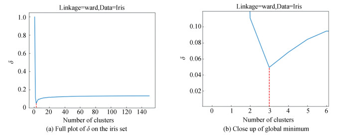
We apply external validation to the iris data set from the UC Irvine Machine Learning Repository, which has three natural classes that form the reference partition
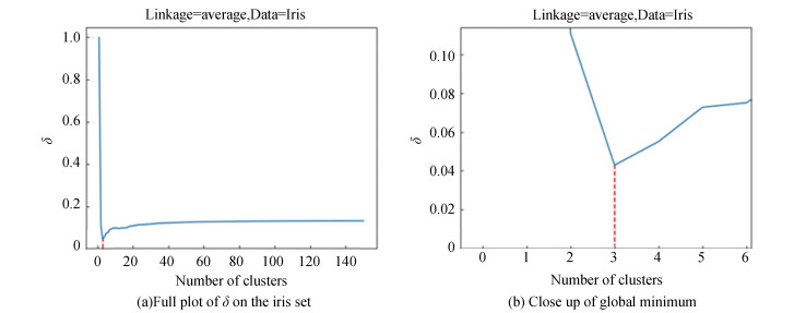
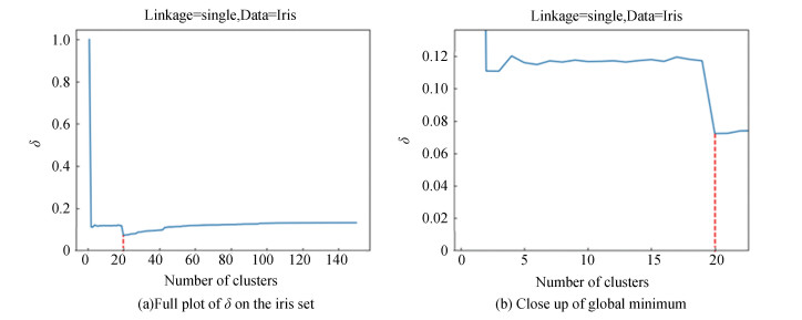
We focus primarily on the Ward method clustering method, depicted in Fig. 3, given its relevance to our theoretical framework. We also include plots for complete, single, and average link methods for comparison in Figs. 4 and 5, respectively. Each plot includes a vertical dashed line denoting the number of clusters at which the
|
Fig.3
The values of |
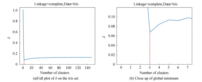
|
Fig.4
The values of |
|
Fig.5
The values of |
If the chosen clustering method is suitable for a specific data set, our results show that a remarkable coincidence with the real number of clusters given in the description of the data set. Also, our results coincide with the experimental results obtained in Ref.[25]. However, when we apply the single-link technique to the iris data set, the minimum distance between the reference partition
|
Fig.6
The values of |
We also note that the Ward and average link methods had the smallest minimum values of the
The

|
Fig.7
The values of |
|
Fig.8
The values of |
|
Fig.9
The values of |
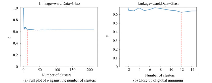
|
Fig.10
The values of |

|
Fig.11
The values of |
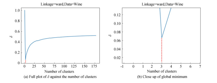
|
Fig.12
The values of |
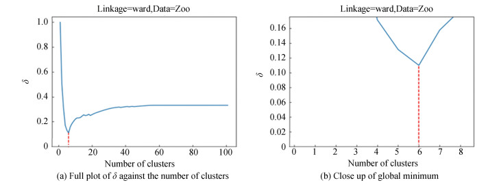
|
Fig.13
The values of |
After pre-processing, each set was clustered according to the Ward hierarchical method and its
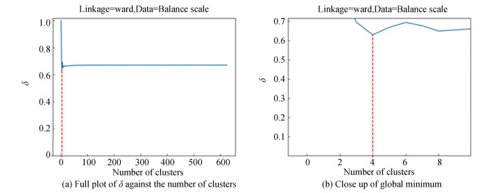
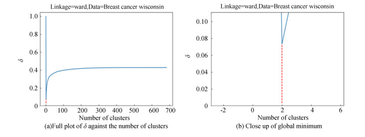
In the majority of the experimental cases, the global minimum of
In zoo, the global minimum is at 6 instead of 7 clusters. This behavior is in part due to the imbalance between the number of elements in each cluster of the true partition, which has seven clusters having 41, 20, 5, 13, 4, 8, and 10 elements.
The behavior of
Balance scale is similarly unevenly weighted, with its cluster sizes being 49, 288, and 288. This seems to suggest that the
| Table 2 Experimental results on several data sets |
The three data sets, zoo, glass, and balance scale, which did not have a minimum
Experimental results suggest that when the data set is not severely imbalanced in cluster size, and a suitable hierarchical linkage method is used, the
We introduced axiomatically the notion of inertial entropy for partitions of data sets that are subsets of a metric space and the conditional variant of this type of entropy. Conditional entropy generates a metric on the space of partitions and this metric can be normalized such that it ranges in the interval [0, 1]. Then, we demonstrate that the partition metric can be used for comparing a reference partition of labeled data with partitions produced by a variety of clustering methods which allows us to evaluate various clustering methods as well as the clusterability of a data set.
It appears that the entropic approach introduced here can be extended to other types of data sets, in particular to graph data sets. This would allow external validation of clusterings of this type of data, a topic for future research.
| [1] |
Simovici D A, Jaroszewicz S. An axiomatization of partition entropy. IEEE Transactions on Information Theory, 2002, 48(7): 2138-2142. DOI:10.1109/TIT.2002.1013159 (  0) 0) |
| [2] |
Simovici D A. Clustering-Theoretical and Practical Aspects. Singapore: WorldScientific, 2021.
(  0) 0) |
| [3] |
Verma R, Merigó J M. On Sharma-Mittal's entropy under intuitionistic fuzzy environment. Cybernetics and Systems, 2021, 52(6): 498-521. DOI:10.1080/01969722.2021.1903722 (  0) 0) |
| [4] |
Boffa S, Ciucci D. Logical entropy and aggregation of fuzzy orthopartitions. Fuzzy Sets and Systems, 2023, 455: 77-101. DOI:10.1016/j.fss.2022.07.014 (  0) 0) |
| [5] |
Chen C, Rajapakse I. Tensor entropy for uniform hypergraphs. IEEE Transactions on Network Science and Engineering, 2020, 7(4): 2889-2900. DOI:10.1109/TNSE.2020.3002963 (  0) 0) |
| [6] |
Birkhoff G. Lattice Theory. 3rd edn. Providence, RI : American Mathematical Society, 1973.
(  0) 0) |
| [7] |
Khinchin A I. Mathematical Foundations of Information Theory. New York: Dover, 1957.
(  0) 0) |
| [8] |
Faddeev D K. On the notion of entropy of finite probability distributions (in Russian). Usp. Mat. Nauk, 1956, 11: 227-231.
(  0) 0) |
| [9] |
Ingarden R S, Urbanik K. Information without probability. Coll. Math., 1962, 1: 281-304. (  0) 0) |
| [10] |
Daróczy Z. Generalized information functions. Information and Control, 1970, 16: 36-51. DOI:10.1016/S0019-9958(70)80040-7 (  0) 0) |
| [11] |
Havrda J H, Charvat F. Quantification methods of classification processes: Concepts of structural α-entropy. Kybernetica, 1967, 3: 30-35. (  0) 0) |
| [12] |
Tsallis C. Possible generalization of boltzmann-gibbs statistics. Journal of Statistical Physics, 1988, 52: 479-487. DOI:10.1007/BF01016429 (  0) 0) |
| [13] |
Furuichi S, Yanagi K, Kuriyama K. Fundamental properties of tsallis relative entropy. Journal of Mathematical Physics, 2004, 45(12): 4868-4877. DOI:10.1063/1.1805729 (  0) 0) |
| [14] |
Ward J H. Hierarchical grouping to optimize an objective function. Journal of the American Statistical Association, 1963, 58: 236-244. DOI:10.1080/01621459.1963.10500845 (  0) 0) |
| [15] |
Miyamoto S, Abe R, Endo Y, et al. Ward method of hierarchical clustering for non-euclidean similarity measures. Proceedings of the 2015 7th International Conference of Soft Computing and Pattern Recognition (SoCPaR). Piscataway: IEEE, 2015, 60-63. (  0) 0) |
| [16] |
Draszawka K, Szymański J. External Validation Measures for Nested Clustering of Text Documents. Emerging Intelligent Technologies in Industry. Ryżko D, Rybiński H, Gawrysiak P, et al. Heidelberg: Springer Berlin, 2011: 207-225. DOI: 10.1007/978-3-642-22732-5.
(  0) 0) |
| [17] |
Brun M, Sima C, Hua J, et al. Model-based evaluation of clustering validation measures. Pattern Recognition, 2007, 40(3): 807-824. DOI:10.1016/j.patcog.2006.06.026 (  0) 0) |
| [18] |
Liu Y, Li Z, Xiong H, et al. Understanding of internal clustering validation measures. Proceedings of the 2010 IEEE International Conference on Data Mining. Piscataway: IEEE, 2010, 911-916. DOI:10.1109/ICDM.2010.35 (  0) 0) |
| [19] |
Wu J, Chen J, Xiong H, et al. External validation measures for k-means clustering: A data distribution perspective. Expert Systems with Applications, 2009, 36(3): 6050-6061. DOI:10.1016/j.eswa.2008.06.093 (  0) 0) |
| [20] |
Ullmann T, Hennig C, Boulesteix A-L. Validation of cluster analysis results on validation data: A systematic framework. Wiley Interdisciplinary Reviews: Data Mining and Knowledge Discovery, 2022, 12(3): 1444. DOI:10.1002/widm.1444 (  0) 0) |
| [21] |
Halmos P R. Lectures on Boolean Algebras. New York: Springer, 1974.
(  0) 0) |
| [22] |
Xiong H, Li Z. Clustering Validation Measures. Data Clustering. Aggarwal C C, Reddy C K. New York: CRC Press, 2018: 571-606.
(  0) 0) |
| [23] |
Pal N R, BiswasJ. Cluster validation using graph theoretic concepts. Pattern Recognition, 1997, 30(6): 847-857. DOI:10.1016/S0031-3203(96)00127-6 (  0) 0) |
| [24] |
Schubert E. Stop using the elbow criterion for k-means and how to choose the number of clusters instead. ACM SIGKDD Explorations Newsletter, 2023, 25(1): 36-42. DOI:10.1145/3606274.3606278 (  0) 0) |
| [25] |
Arbelaitz O, Gurrutxaga I, Muguerza J, et al. An extensive comparative study of cluster validity indices. Pattern Recognition, 2013, 46(1): 243-256. DOI:10.1016/j.patcog.2012.07.021 (  0) 0) |
| [26] |
Milligan G W, Cooper M C. An examination of procedures for determining the number of clusters in a data set. Psychometrika, 1985, 50: 159-179. DOI:10.1007/BF02294245 (  0) 0) |
 2024, Vol. 31


