Abstract
The inherent nonlinearity and time-delay characteristics of industrial refrigeration processes complicate parameter tuning for conventional PID control, adversely affecting its precision. This makes the control of such systems a significant and challenging research problem. To address this, a novel Neural Network Predictive Control (NNPC) algorithm is proposed, which integrates an Improved Deep Belief Network (IDBN) with an Improved Whale Optimization Algorithm (IWOA). First, the IDBN acts as a high-precision nonlinear prediction model, significantly improving multi-step prediction accuracy. Second, the IWOA is employed to optimize the predictive controller, featuring three major improvements: an improved population initialization, a modified convergence factor update mechanism, and an added disturbance strategy, which collectively accelerate convergence and enhance global search capability. Finally, simulation results demonstrate that the proposed NNPC algorithm achieves superior set-point tracking performance and strong robustness against external disturbances.
0 Introduction
Industrial refrigeration processes achieve multiple critical functions through temperature control, holding profound significance for industrial production, product quality, and environmental protection. Industrial refrigeration processes inherently exhibit nonlinear dynamics with time-delay characteristics. The conventional PID control method struggles to achieve satisfactory control performance due to the difficulties in parameter tuning. Consequently, the control of nonlinear time-delay refrigeration systems has emerged as a significant research focus, garnering increasing attention from scholars [1-2]. Model Predictive Control(MPC) integrates rolling optimization, multi-step prediction and feedback correction, and it has been widely studied in industrial process control for its good control performance and strong robustness [3-5]. Industrial refrigeration processes achieve temperature control through MPC, which avoids the lag and oscillations caused by traditional PID control. Its ability to handle constraints ensures the system always operates within safe limits.
The MPC method typically employs linear models to approximate these nonlinear time-delay systems. However, predictions based on such simplified linear models often lead to degraded control accuracy. In recent years, Neural Network Predictive Control(NNPC) has attracted increasing research attention in the field of nonlinear predictive control algorithms due to its excellent nonlinear approximation ability [6-10]. A data-driven sparse regression-based identification method combined with MPC was proposed in Ref.[6]. This data-driven framework accurately captures system nonlinearities with low forecasting error, enabling smooth control input changes and nonlinear MPC strategies for adaptable large-scale water management. A partially connected Recurrent Neural Network(RNN) with generalized error bounds was developed to approximate a nonlinear dynamic system in Ref.[7]. This prediction model can reduce the mean square error of multi-step prediction, furthermore, the control input changes smoothly and oscillations are less in the closed-loop simulation. A NNPC method based on two sets of Radial Basis Function Neural Networks(RBFNNs) was provided in Ref.[8]. One set of RBFNNs is used as the prediction model, and the other set is used to solve optimization problems. The proposed predictive controller has good tracking performance for the robotic arm. However, a critical limitation persists in existing studies: enhancing multi-step prediction performance without increasing the architectural complexity of traditional shallow neural networks remains an unresolved challenge. Recently, the excellent predictive performance of deep learning algorithms has gained widespread attention. In Ref.[9], a trajectory prediction model based on Long Short Time Memory(LSTM) deep learning and an MPC algorithm were used to achieve trajectory prediction and tracking of intelligent ships under mixed wind and current disturbances. The proposed LSTM deep learning method has better accuracy and reliability than the traditional methods. Ref.[10]reported a predictive control method based on the Deep Belief Network(DBN) deep learning model of time series to solve the problems of time-delay, nonlinearity and high data complexity in the denitrification system, achieving more accurate prediction of NOx emissions. The rolling optimization solution of the optimal control input is based on the differential evolution algorithm. The proposed method not only has higher control precision but also can save the amount of raw materials. Due to the nonlinearity and time-delay in industrial refrigeration systems, improving deep learning algorithms' prediction accuracy remains an open research problem.
Another challenge in current NNPC research is developing real-time optimization algorithms that efficiently solve the nonlinear programming problems within each control cycle [11-14]. Ref. [11]adopted feedforward neural network as a multi-step prediction model and Tent mapped chaos optimization algorithm was applied to the nonlinear rolling optimization, which improves the convergence and accuracy. Ref.[12] designed a new training and optimization method that combines the steps of data generation and neural network training into a high-dimensional stochastic optimization problem that effectively solves large-scale optimization problems using parallel computing techniques, enabling MPC to be applied to nonlinear system control in real time. Ref.[13]formulated the performance indicator function in nonlinear MPC as a convex nonlinear minimization problem, which was transformed into a constrained Quadratic Programming(QP) problem, and the general projection neural network was applied to solve this QP to obtain the optimal solution. Fuzzy Sequential Quadratic Programming(SQP) algorithm was studied to design the rolling optimization controller in Ref.[14], which can avoid the problem that SQP algorithm is easy to fall into a local optimum. However, improving the optimization algorithm to promote its convergence speed and search capability remains a challenging problem.
Based on the above analysis, aiming to address the nonlinear and time-delay control problem in industrial refrigeration processes, a novel NNPC algorithm based on IDBN(Improved Deep Belief Network) deep learning and the IWOA(Improved Whale Optimization Algorithm) algorithm is proposed in this paper. The IDBN deep learning algorithm based on DBN and Extreme Learning Machines(ELM) is proposed, and used as a nonlinear prediction model to improve the accuracy of multi-step prediction. The improved convergence speed and search ability of IWOA result from three aspects: replacing the initial population, changing the iterative mode of convergence factor and adding disturbance strategy. Simulation results demonstrate that the proposed NNPC method achieves superior set-point tracking performance and strong robustness against external disturbances. The contributions of this paper are as follows:
1) An IDBN algorithm based on DBN and ELM is proposed, which integrates the powerful feature extraction capability of DBN and the fast learning speed of ELM. The IDBN acts as a high-precision nonlinear prediction model, significantly improving multi-step prediction accuracy.
2) An IWOA optimization algorithm is proposed to promote the convergence speed and search ability from three aspects: replacing the initial population, changing the iterative mode of convergence factor and adding a disturbance strategy.
3) A NNPC algorithm based on IDBN deep learning and IWOA is proposed to improve the control effect of the industrial refrigeration process. The simulation results show that the proposed NNPC algorithm has better control effects in the case of set point tracking control and the presence of disturbance in industrial refrigeration process.
The rest of this paper is organized as follows. Section 1 introduces the proposed IDBN algorithm. Section 2 describes the IWOA algorithm. Section 3 describes the design of the proposed NNPC algorithm. Section 4 conducts the simulation and results analysis of NNPC in industrial refrigeration processes. The conclusion will be given in Section 5.
1 IDBN Algorithm
1.1 Restricted Boltzmann Machine
As a kind of deep learning algorithm, DBN adopts unsupervised layer-by-layer training and supervised backward fine-tuning, which can effectively avoid the problem of long training time and falling into local optimum of neural networks due to random initialization of parameters. The basic module of DBN is Restricted Boltzmann Machine(RBM)[15-16], as shown in Fig.1. The structure of an RBM is composed of two layers of neurons, known as the visible and hidden layers. The visible layer represents the features of the input data, while the hidden layer, also called the data feature extraction layer, is used to obtain the relationships between interconnected neurons. The neurons in the visible and hidden layers satisfy the relationship of no connections within layers and full connections between layers.
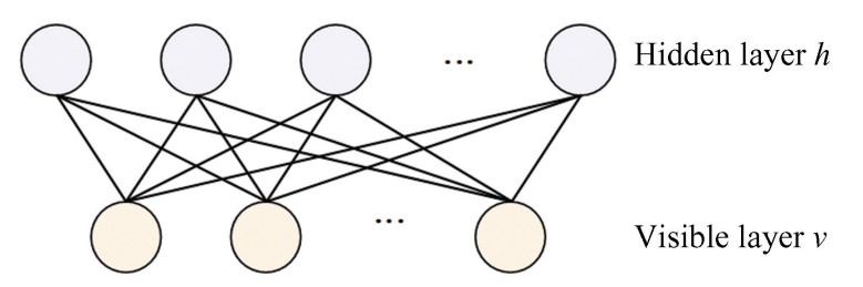
Fig.
1
Schematic diagram of RBM
In Fig.1, it is assumed that the number of neurons in the visible layer is 𝑚𝑣, the number of neurons in the hidden layer is 𝑛ℎ, and the connection weight between the ith visible layer neuron and the jth hidden layer neuron is 𝑤𝑖𝑗, 𝑏𝑖 and 𝑎𝑗 represents their biases, respectively. For the given 𝑣 and ℎ, the energy function of RBM can be expressed as follows:
(1)
The network assigns a probability to each possible visible-hidden vector pair through an energy function, as shown in Eq.(2):
(2)
where Z is obtained by summing over all possible visible-hidden vector pairs:
(3)
The probability of the model assigned to the visible vector 𝑣 is:
(4)
As RBM adopts the form of no connections within layers and full connections between layers, the activation probabilities of neurons are independent of each other. The calculation equation is as follows:
(5)
(6)
where 𝜎(𝑥)=(1+e-𝑥)-1. The input vector of RBM is the external data received through the visible layer, which is transmitted to the hidden layer through the activation function. In other words, the data vector obtained by the hidden layer can be regarded as feature representations of the original input vector.
The calculation of parameters in RBM is determined by minimizing the energy function. Given model parameters, the logarithmic probability of training data can be expressed as:
(7)
Make the set of parameters 𝜓={ 𝑊,𝑏,𝑎}, the result of taking the partial derivative of lo𝗀 𝑝(𝑣) over 𝜓 is:
(8)
According to Eq.(8), the update rule for parameters is:
(9)
where<·>data represents the expected value of the original data, 𝜂 represents the learning rate, and<·>model represents the expected value of the model, calculated by the contrastive divergence method.
1.2 Deep Belief Network
The DBN is composed of multiple RBMs stacked [17-18], and its structure diagram is shown in Fig.2. The hidden layer of the former RBM is the visible layer of the latter RBM, which is stacked on top of each other to form a DBN model containing multiple hidden layers. In the RBM stack, unsupervised learning is used to train the whole network structure. The data processed by RBM at the top layer is used as the input data of BP(Back Propagation) neural network, and the BP neural network is used for training and output data. The error between the predicted value and the expected value of the output is calculated, and the error is backpropagated, so as to fine-tune the global network parameters and optimize the output prediction.
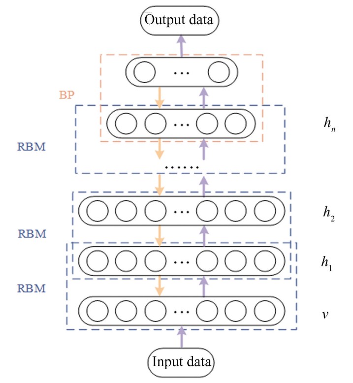
Fig.
2
DBN model structure
1.3 IDBN Algorithm
The DBN top layer uses BP neural network to output the predicted values. However, the shortcomings of BP neural network, such as its sensitivity to initial network weights and slow convergence speed, cannot be ignored. ELM is a machine learning method based on feedforward neural network construction. The algorithm calculates the corresponding output weights by randomly initializing input weights and biases, and the weights do not need to be adjusted iteratively. The reduction of a large number of operations makes ELM algorithm have a faster learning speed than traditional BP learning algorithms. Different from traditional BP learning algorithms that focus only on achieving the minimum training error, ELM algorithm also tends to minimize the weight norm, so it has better generalization ability [19-20]. Combining the feature extraction capability of DBN with the advantages of fast learning speed and good generalization ability of ELM, the proposed IDBN algorithm is shown in Fig.3. As an ELM neural network structure with fast learning speed, the improved IDBN model architecture effectively overcomes the aforementioned issues of the classical DBN.
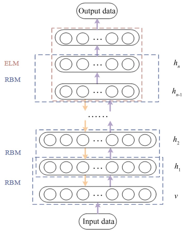
Fig.
3
IDBN algorithm structure
Firstly, the greedy algorithm is used to train the neural network containing 𝑛 hidden layers layer by layer, and then the BP algorithm is used to optimize the parameters of the whole network from top to bottom, so as to update the parameters of all RBMs to the optimal states. Considering the hidden layer ℎ𝑛-1, ℎ𝑛 and the output layer as a typical ELM structure, the input weights and biases of the ELM can be initialized using the parameters of the topmost RBM layer obtained to calculate the output weights of the ELM.
Suppose the input of the ELM network is 𝑥𝑗 and the output is 𝑡𝑗, 𝑗=1,2,···,𝑙. The ELM output function with 𝑆 hidden layer neurons is expressed as follows:
(10)
where 𝛽𝑖 denotes the output weight of the 𝑖th hidden layer neuron to the output neuron, 𝐺(𝑥) denotes the Sigmoid activation function, the input weights and biases of the ELM{𝑊𝑖,𝑏𝑖,𝑖=1,2,···,𝑆} can be obtained from the topmost RBM parameters of DBN. Eq.(10) can be written in matrix form as follows:
(11)
where
(12)
(13)
in which 𝑯 represents the output matrix of the hidden layer, also termed the ELM feature space. The ELM training process involves finding the optimal output weight matrix , that is, to find the least squares solution , so that:
(14)
When 𝑯 is the full rank of the column, using the Moore-Penrose generalized inverse, we can obtain:
(15)
where 𝑯†=(𝑯T𝑯)-1𝑯T. When the output matrix of hidden layer is not column full rank, the optimal output weight matrix can be obtained by using the singular value decomposition method.
DBN-ELM model contains many parameters, and improper parameter selection will cause the algorithm to converge on the local optimal solution, which directly affects the feature extraction ability and generalization of the network. Therefore, an Equilibrium Optimizer(EO) algorithm is proposed to determine the parameters in the DBN-ELM network [21-22].
The flow chart of the IDBN model algorithm is shown in Fig. 4.
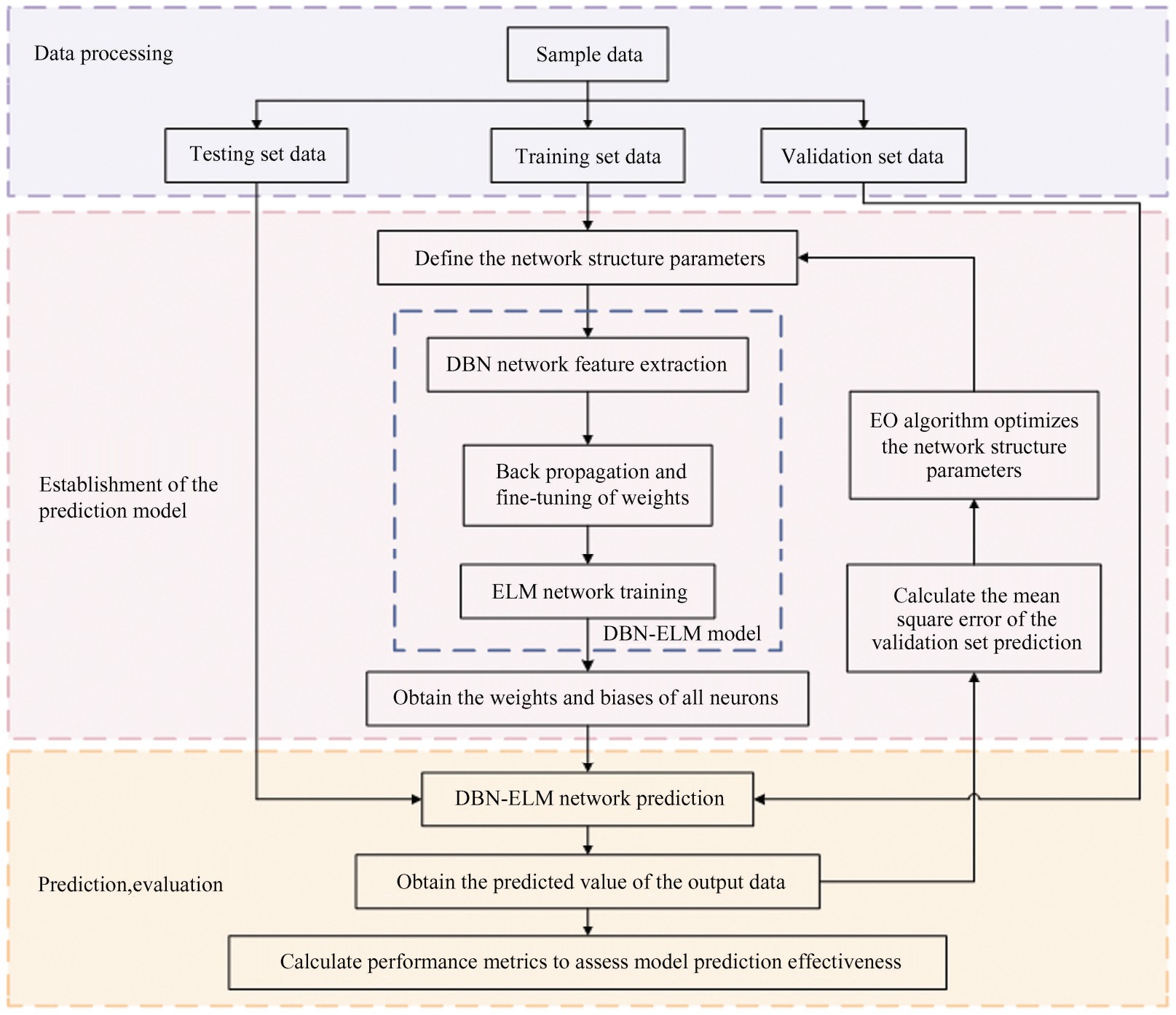
Fig.
4
Flow chart of IDBN algorithm
The specific training procedure of the IDBN algorithm is as follows. After the data is split into training, validation, and testing set, the EO algorithm randomly initializes a set of solutions, trains RBMs layer by layer according to the training set data, and finally uses the BP algorithm for weight fine-tuning. The weight and bias of the topmost RBM serve as the input weight and bias of ELM algorithm, thus getting the output weight matrix of ELM. Then the prediction output of ELM algorithm is realized. EO algorithm takes the mean square error of the validation set prediction results as the objective function, iterates constantly to minimize it, and outputs the optimal network structure parameters. The whole DBN-ELM network is retrained according to the training set data and the optimized network structure parameters. The test set prediction results are used to calculate the performance index and to evaluate the performance of the whole network.
2 IWOA Algorithm
2.1 Whale Optimization Algorithm
The hunting mechanism of humpback whales serves as the inspiration for the Whale Optimization Algorithm(WOA) [23-24]. Bubble net feeding is a species-specific foraging behavior of humpback whales. Near the surface, humpback whales commonly prey upon groups of krill or small fish, and this foraging has been observed to be accomplished by creating distinctive bubbles in the circular path shown in Fig. 5. In the WOA algorithm, the mathematical model is constructed based on three behaviors: bubble-net attacking, rounding up prey, and random prey searching [25-26].
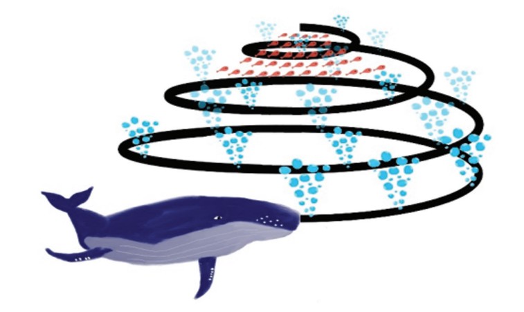
Fig.
5
Humpback whales' bubble-net feeding behavior
Since the NNPC performs the optimization process once at each sampling moment, the fast convergence of the optimization algorithm and its searching ability are particularly important. In this paper, the proposed IWOA is to promote the convergence speed and search ability of whale optimization algorithm from three aspects: replacing the initial population, changing the iterative mode of convergence factor and adding disturbance strategy.
1) Rounding up prey. In this behavioral model, humpback whales encircle the prey after locating it. Similarly, in the WOA, each whale is modeled as an individual whose position in the search space constitutes a potential solution. Since the true optimal solution is unknown, the WOA designates the current best solution as the target prey. All other individuals then update their positions to move closer to this target, as defined by the equation below:
(16)
(17)
where and are coefficient vectors, 𝑖 is the current iteration number, (𝑖) is the current position vector, best(𝑖) is the position vector of the optimal solution obtained in the 𝑖th iteration. The coefficient vector and can be calculated by the equation below:
(18)
(19)
where is a control parameter that decreases linearly from 2 to 0 as iterations proceed, denotes a random vector in [0,1].
2) Bubble-net attacking. The bubble-net feeding behavior of humpback whales is characterized by an upward spiral path. Accordingly, two mathematical approaches are devised to simulate the spiral bubble-net feeding strategy.
Shrinking the surround mechanism: This is achieved by linear reduction of in Eq.(18), and the variation range of is also narrowed accordingly. Since is a random value in [-𝑎,𝑎], when takes a random value between [-1,1], the new location of the search agent can be defined as any location between the current location and the prey location.
Spiral updating position: The distance between the whale and prey is used to establish a spiral position equation, replicating the humpback whales' spiral hunting motion.The mathematical formula is calculated as follows:
(20)
(21)
where 𝑏 is the parameter governing the logarithmic spiral's geometry, is the distance between the 𝑗th whale and the prey, 𝑙 is a random number in [-1,1].
Humpback whales swim in a spiral trajectory along progressively smaller circles when hunting. To simulate this behavior, assume that during optimization, the humpback whale has a 50% probability of updating its coordinates by shrinking the surrounding area and spiraling to a new position. The specific expression is as follows:
(22)
where 𝑝 is a random number in [0,1].
3) Random search for prey. Variations of can also be used to find prey. When the random value of is greater than 1 or less than-1, the search agent will stay away from the reference whale. At this stage, the algorithm selects a random search agent to guide the search, rather than choosing the optimal search agent to date as in the previous stage. This mechanism enhances the global search capability of the WOA algorithm. The specific expression is as follows:
(23)
(24)
in which rand is a random position vector denoting a whale chosen randomly from the current population.
2.2 Tent Map Initializes the Population
Chaotic mappings are used to generate chaotic sequences, and chaotic sequences with ergodicity and randomness can usually obtain more uniform and diverse solutions than pseudo-random number distributions in the search space. In this paper, Tent map is used to initialize population to improve the diversity of initial solutions of whale optimization algorithm and to speed up the algorithm convergence. The way that Tent map generates a random sequence is as follows:
(25)
in which 𝑖=1,2,···,𝑛IWOA, 𝑛IWOA is the population size, 𝑧(1) is a random number not equal to 𝛼𝑇, take 𝛼𝑇=0.499.
2.3 Nonlinear Convergence Factor
The value of the convergence factor 𝑎 in the whale optimization algorithm determines whether the algorithm adopts the current optimal solution to guide the search or randomly selects a search agent to guide the search, that is, the value of 𝑎 affects the local and global search performance of the algorithm. In this paper, a nonlinear change in the value of convergence 𝑎 is used to replace the linear convergence in the traditional WOA algorithm in order to make the value of 𝑎 decay faster at the beginning of the iteration to achieve the fast convergence of the algorithm, and the slow change of 𝑎 at the end of the iteration can further improve the local search ability of the algorithm. The equation for the nonlinear convergence of the convergence factor 𝑎 with the number of iterations is shown as follows:
(26)
where 𝑐max_iter is the maximum iteration count, 𝑡 is the current iteration number, 𝜌 is a constant greater than 1, 𝜌=3.
2.4 Levy Flight Disturbance Strategy
In this paper, a Levy flight disturbance strategy is introduced after the location update of the search agent, so that individual whales can explore a larger search space and avoid falling into local optimization, and further improve the global optimization ability of the algorithm. Levy flight is a random wandering strategy, which is a random search method subject to Levy distribution. Since the position of Levy flight is updated in such a way that steps of short distance and occasionally longer distance are spaced apart, the method can explore a larger space than Brownian motion for the same number of steps or distance [27]. The equation for Levy flight disturbance strategy to update the search agent location is as follows:
(27)
where (𝑡) represents the location of the search agent after updating with the Levy flight disturbance strategy, (𝑡) represents the location of the current search agent, 𝜎 is the weight that controls the step, 𝜎=1, ⊕ denotes point-to-point multiplication, and Levy(λ) represents a path that obeys Levy distribution, satisfied Levy(λ)~ 𝑢=𝑡-λ,1<λ<3.
Mantegna algorithm is used to simulate the random step size 𝑠 of Levy distribution. The equation is shown as follows:
(28)
where 𝜃=1.5, 𝜇 and 𝜐 follow normal distributions 𝜇~𝑁(0,) and 𝜐~𝑁(0,), with variances of
(29)
To ensure that the current search agent's fitness is optimal, a greedy algorithm is used to decide whether to update the whale's position. It is expressed in the following equation:
(30)
2.5 IWOA Algorithm
The flowchart of the proposed IWOA algorithm is shown in Fig. 6. The IWOA algorithm is calculated as follows. Firstly, the population is initialized using Tent map to obtain more evenly distributed and diverse initial solutions. The IWOA algorithm begins with a set of random solutions. In each iteration, it may select either the random search agent or the current best search agent to guide the search process. The IWOA algorithm dynamically selects between a spiral update and a shrinking encirclement based on the value of 𝑝. In the process of iteration, decreases nonlinearly from 2 to 0, and the range of variation for is correspondingly reduced. When||<1, selecting the current optimal solution to guide the search. When||>1, selecting the random search agent to guide the search. After the search agent position is updated, Levy flight disturbance strategy is introduced to enable individual whales to explore a larger search space. The location of the search agent is updated to ensure that the fitness of the current search agent is optimal. Upon reaching the maximum iteration count, the IWOA algorithm outputs the optimal parameter values.
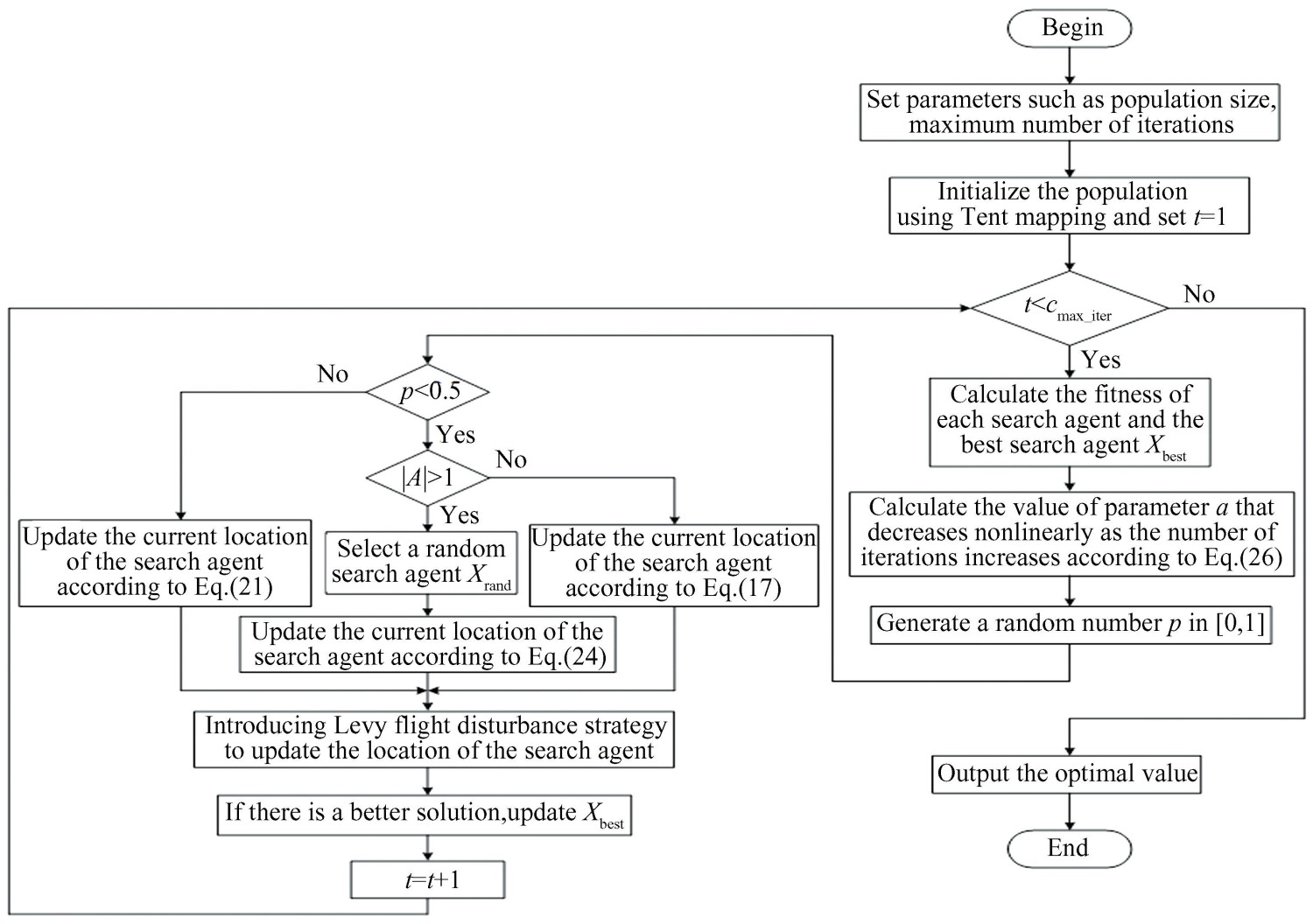
Fig.
6
Flow chart of IWOA algorithm
3 NNPC Algorithm
The combination of neural networks and predictive control plays an important role in the control of industrial processes such as nonlinear and time-delay [28-29]. The proposed IWOA-IDBN-NNPC algorithm in this paper is shown in Fig.7. Firstly, the IDBN neural network model is proposed, which predicts the system's future output based on historical control inputs, actual system outputs, and future control inputs. Then, the error between the output prediction obtained after feedback correction and the reference trajectory is calculated. IWOA algorithm is proposed to roll optimize the performance indicators related to this error.
In the actual control system, drastic changes in the control input and output are often not expected. Online softening processing of the set point can obtain a relatively gentle reference trajectory, so that the output 𝑦(𝑘) reaches the set point along a smooth curve. In this paper, the setting for the softened reference trajectory is as follows:
(31)
where 𝑦𝑟(𝑘+𝑗) represents the expected reference trajectory, 𝑦(𝑘) is the actual system output at the current moment, 𝑅(𝑘) is the set point, 𝛼𝑟 is the softening coefficient and 𝛼𝑟=0.6.
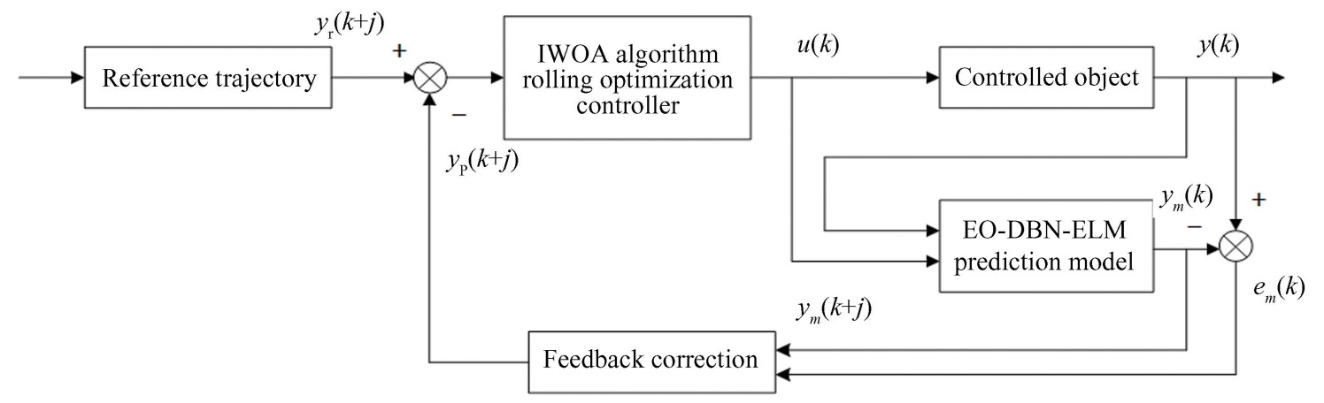
Fig.
7
Neural network predictive control architecture
Recursive multi-step prediction is adopted in this paper, the IDBN model is used for each prediction, and the actual output of the system at future time is replaced by the predicted output [30]. Suppose that the established neural network model is 𝑓𝑁𝑁[·], the output prediction of the system at the next moment can be expressed as:
(32)
where 𝑦𝑚(𝑘+1) represents the current prediction output, 𝑦(𝑘) is the actual system output at the current moment, 𝑢(𝑘) is the input, 𝜉(𝑘) denotes the Gaussian white noise sequence with zero mean.
Replacing the unknown 𝑦(𝑘+1) in the second step prediction input with the current prediction output 𝑦𝑚(𝑘+1), then:
(33)
If the prediction time domain 𝑃 and the control time domain 𝐿 are known, the 𝑃th step prediction can be expressed as:
(34)
in which [𝑢(𝑘),𝑢(𝑘+1),···,𝑢(𝑘+𝐿-1)] is the control input of the output of the 𝑘-step rolling optimization. When 𝑃>𝐿, replace the control input that has not been determined with 𝑢(𝑘+𝐿-1).
The feedback correction link is introduced to correct or compensate the prediction model output, preventing it from deviating from the actual system output. The error between the actual system output and the prediction model output is first calculated as follows:
(35)
The corrected output prediction is:
(36)
where 𝑗=1,2,···,𝑃, 𝜒 is the error correction coefficient, and 𝜒=0.5.
The trajectory tracking error, derived from the reference and the predicted output, is computed as follows:
(37)
The role of rolling optimization is to obtain an optimal set of control inputs by minimizing a certain performance index containing 𝑒𝑃(𝑘+𝑗). In order to make the control input as stable as possible, the variation of the control input is introduced into the performance index function, which is specifically expressed as follows:
(38)
where 𝜒1 is the error weight coefficient, 𝜒2 is the control weight coefficient, take 𝜒1=1.0, 𝜒2=0.6. In this paper, IWOA algorithm is used to optimize the performance index 𝐽 at each sampling moment, which can output the optimal control input.
4 Simulation Results and Analysis
In this section, the proposed IWOA-IDBN-NNPC algorithm is simulated and compared with WOA-IDBN-NNPC in terms of their capabilities in reference tracking and interference suppression. Control of a nonlinear system and nonlinear time-delay industrial refrigeration processes are considered here.
Overshoot 𝜎% and Integral of Squared Error(𝐼ISE) are adopted as performance evaluation indices for the NNPC control system. The calculation equations are as follows:
(39)
(40)
where 𝑦𝑝 indicates the peak value of step response, 𝑦𝑠 indicates steady-state value, 𝑒(𝑡) indicates the deviation of the system output from the set point.
4.1 Simulation Results of the IWOA Algorithm for Benchmark Functions
In this section, we first evaluate the convergence and search capability of the proposed IWOA, with comparative analysis against the original WOA algorithm results. Three benchmark test functions, namely single-peak test function 𝐹3, multi-peak test function 𝐹8 and fixed-dimension multi-peak test function 𝐹22, are selected for simulation experiments. Their equations are as follows:
(41)
(42)
(43)
The three-dimensional surface diagram of the three functions is shown in Fig.8. Setting the population size as 30 and the maximum number of iterations as 50, the results of IWOA and WOA algorithms for finding the optimum are shown in Fig. 9. Compared with the WOA algorithm in Fig. 9, the proposed IWOA algorithm converges more quickly at the beginning of the iteration and can find the optimum solution with lower adaptation. Experimental results demonstrate that both the convergence speed and optimal solution search capability of the IWOA algorithm have been significantly enhanced.
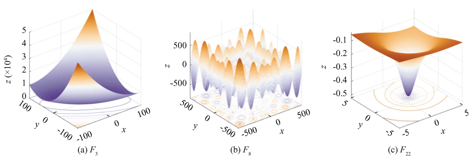
Fig.
8
3D surface diagrams of the benchmark functions
4.2 IWOA-IDBN-NNPC for Nonlinear System
In this section, we compare the control performance of the proposed IWOA-IDBN-NNPC with that of WOA-IDBN-NNPC for a nonlinear system. Suppose the nonlinear system is:
(44)
where 𝑦(·) is the actual system output at different moments, 𝑢(·) is the actual system input at different moments.
The specific experimental parameters were set as follows. Firstly, a set of control inputs with values between [0,1] is randomly generated and the corresponding output data is obtained according to the model. The 1000 sets of data with input [𝑦(𝑘-1),𝑢(𝑘-1),𝑢(𝑘-2)] and output 𝑦(𝑘) are used to construct the prediction model, and the training set, validation set and testing set are divided according to the ratio of 7∶2∶1. The DBN-ELM neural network containing four hidden layers is established. After EO algorithm optimization, the number of neurons in each hidden layer is determined to be 34, 3, 7, and 23, and the number of training RBMs is 100 times. Fig.10 displays the prediction results of the proposed improved IDBN model on the test set. The predicted values in the figure perfectly match the actual sample values. Simulation results demonstrate that the IDBN algorithm proposed in this paper exhibits excellent generalization performance.
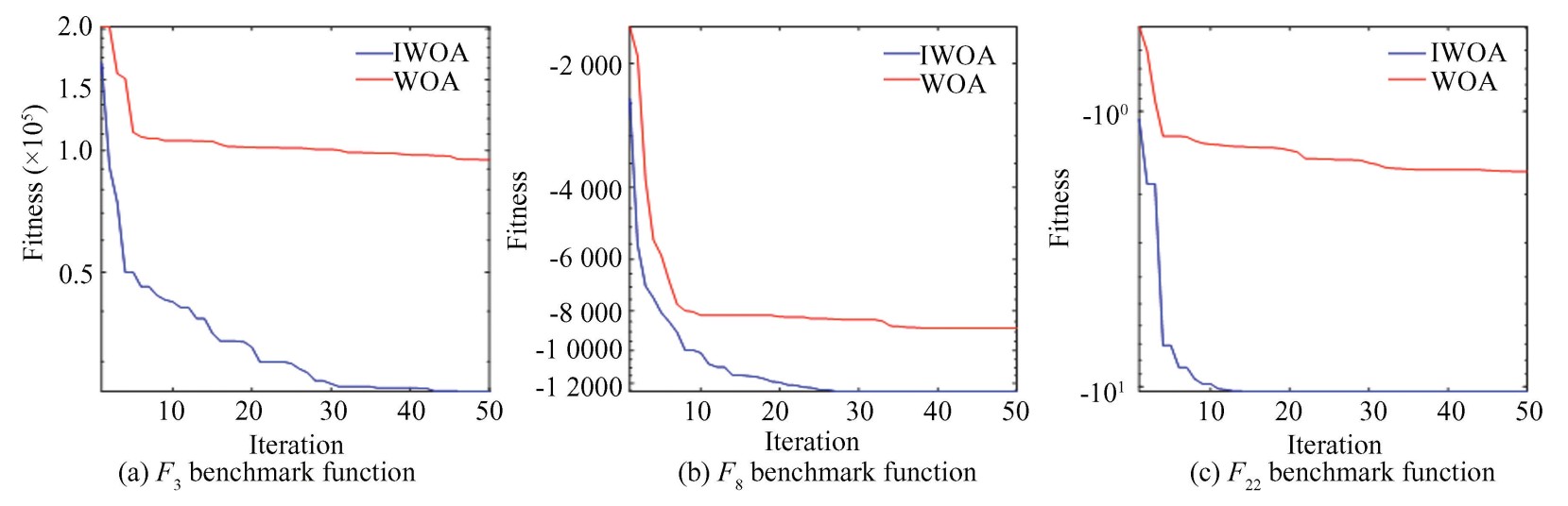
Fig.
9
IWOA and WOA convergence curves of the benchmark functions
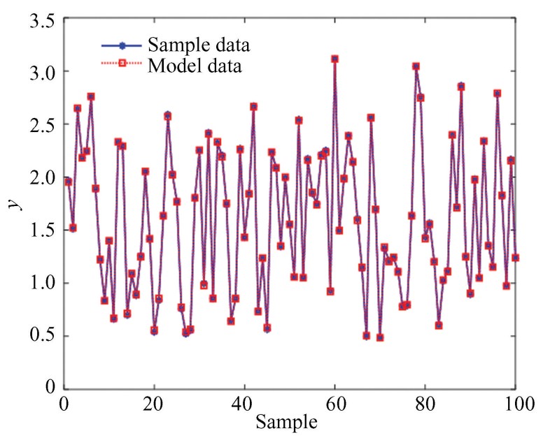
Fig.
10
Prediction results of the proposed IDBN on the testing set
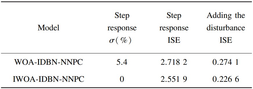
Set the prediction time domain 𝑃=5, the control time domain 𝐿=2, the number of simulation steps to 100, the population size in the optimization algorithm to 30, the maximum number of iterations to 10, and the set point is in square wave form. The simulation results of neural network predictive control using WOA algorithm and IWOA algorithm for optimization are shown in Fig.11 and Fig.12, respectively. In these figurers, 𝑦𝑟(𝑘) denoted the set point change and 𝑦(𝑘) is the controlled variable output. In order to test the anti-disturbance capability of the proposed method, the set point is set to 1 and a disturbance is added at step 50. The simulation results are shown in Fig.13 and the nonlinear system dynamic response indexes are shown in Table 1. From Fig.11 and Fig.12, compared with the WOA algorithm, the actual output of the system after the IWOA algorithm can track the set point more stably, and maintain stability after reaching the set point, with no overshoot, small steady-state residual error and other characteristics, and has a good control effect. From Fig.13 and Table 1, we can also observe that the IWOA-IDBN-NNPC controller demonstrates superior control performance. It recovers to a stable state more rapidly when encountering disturbances and exhibits stronger disturbance rejection capabilities.
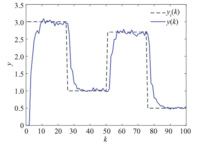
Fig.
11
Simulation results of the WOA-IDBN-NNPC
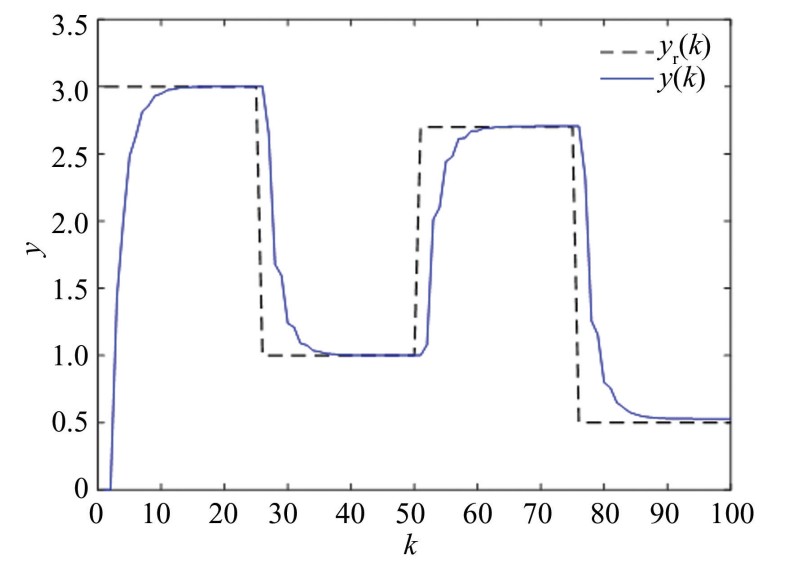
Fig.
12
Simulation results of the IWOA-IDBN-NNPC
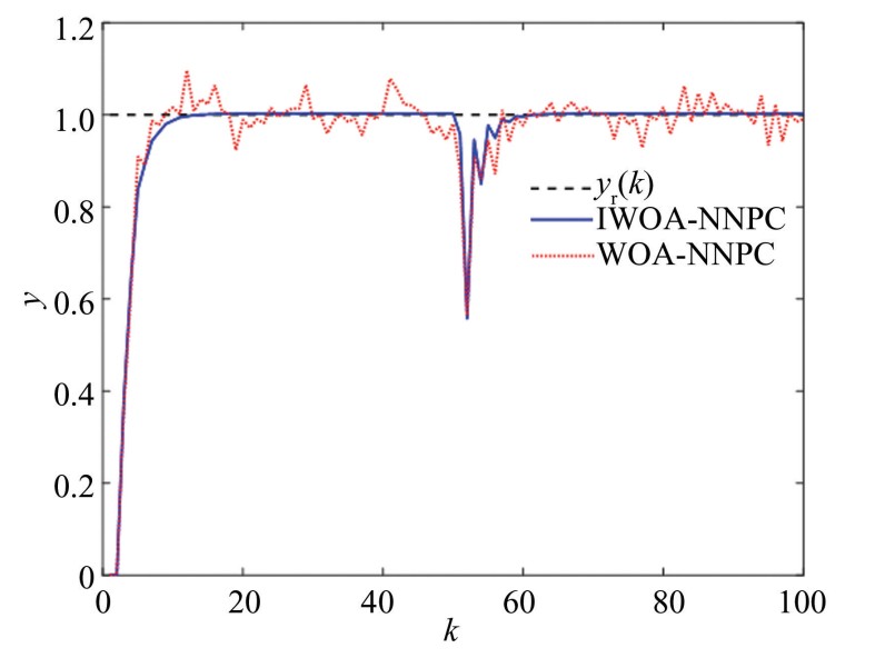
Fig.
13
Comparison of the control effects in the case of adding the disturbance
Table
1
Dynamic response index of the nonlinear model
4.3 IWOA-IDBN-NNPC for Industrial Refrigeration Processes
In this section, a comparison of the control performance between IWOA-IDBN-NNPC and WOA-IDBN-NNPC in nonlinear time-delay industrial refrigeration processes is conducted. A nonlinear time-delay industrial refrigeration process is to be [31]:
(45)
where 𝑦(·) is the actual refrigeration temperature output of the industrial refrigeration process at different moments, 𝑢(·) is the industrial refrigeration process input at different moments, 𝑑 is the process delay 𝑑=26, 𝑎1=0.575 2, 𝑎2=0.230 8, 𝑎3=-0.018 6, 𝑎4=1.109×10⁻⁶, 𝑎5=0.112 7, 𝑎6=-2.775×10⁻⁴.
The specific experimental parameters were set as follows. The value of the control input 𝑢(𝑘) is between [40,80], and the expected output is set to-10. Randomly generate a set of control inputs 𝑢(𝑘) taking values between [40,80], and obtain the corresponding output data according to Eq.(45). The 1000 sets of data with input [𝑦(𝑘-1),𝑦(𝑘-2),𝑦(𝑘-3),𝑢(𝑘-𝑑-3)] and output 𝑦(𝑘) are used to construct the prediction model, and the training set, validation set and testing set are divided according to the ratio of 7∶2∶1. A DBN-ELM neural network containing four hidden layers is established. After EO algorithm optimization, the number of neurons in each hidden layer is determined to be 36, 35, 42, and 50, and the number of training RBMs is 90 times. The prediction results of the proposed IDBN model on the testing set are shown in Fig.14. Simulation results of industrial refrigeration processes also demonstrate that the predicted values in Fig.14 perfectly match the actual sample values, indicating that the proposed IDBN algorithm exhibits outstanding generalization performance.
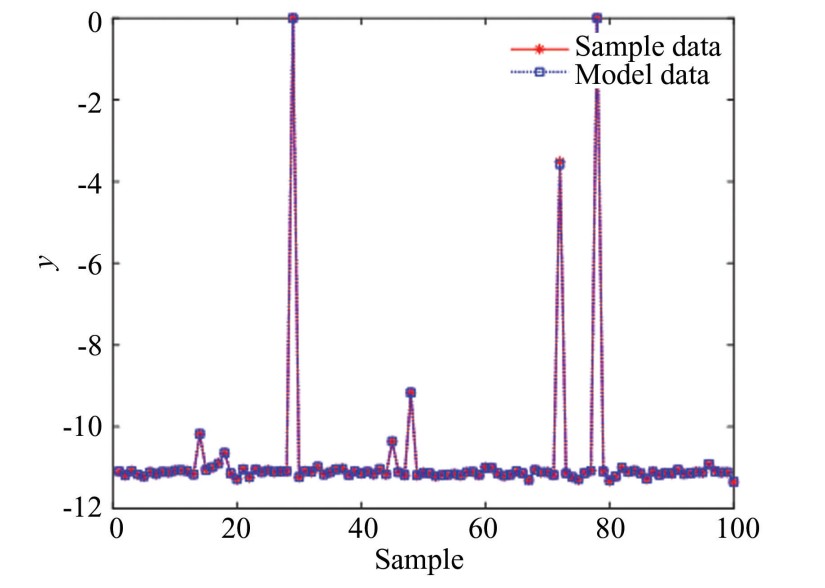
Fig.
14
Prediction results of the proposed IDBN on the testing set
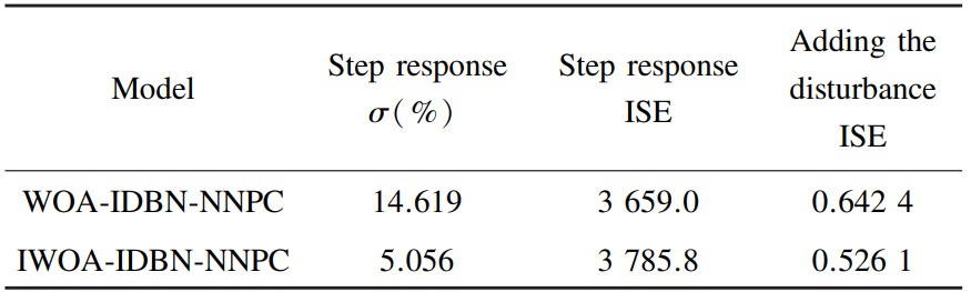
Set the prediction time domain 𝑃=30, the control time domain 𝐿=2, the number of simulation steps to 100, the population size in the optimization algorithm is 30, and the maximum number of iterations is 10. The comparison of the control effects of the two methods is shown in Fig.15. Increasing the disturbance and the simulation results are shown in Fig. 16. The statistical results of the system dynamic response indicators are shown in Table 2. From Fig.15, when IWOA algorithm is used as the optimization controller, the overshoot of the system response is smaller and the system reaches the stable state faster. From Fig.16 and Table 2, the IWOA-IDBN-NNPC controller exhibits minimal overshoot in its setpoint tracking response. When subjected to disturbances, the proposed IWOA-IDBN-NNPC method achieves faster recovery to steady-state conditions. The simulation results demonstrate the effectiveness of the improved IWOA-IDBN-NNPC algorithm proposed in this paper.
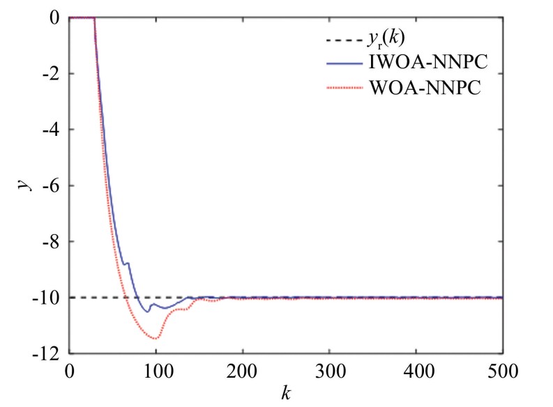
Fig.
15
Comparison of simulation results of nonlinear time-delay model NNPC
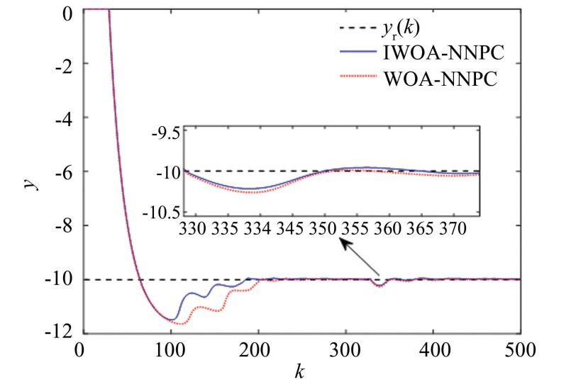
Fig.
16
Comparison of the control effects in the case of adding the disturbance
Table
2
Dynamic response index of the nonlinear time-delay model
5 Conclusions
To control nonlinear and time-delay industrial refrigeration processes, this study proposes a new predictive control algorithm named NNPC, which is based on an IWOA optimization algorithm and an IDBN neural network. The IWOA is enhanced by incorporating a nonlinear convergence factor, Tent chaotic mapping for population initialization, and a Levy flight disturbance strategy. The resulting IWOA exhibits stronger global search capability and faster convergence speed. Meanwhile, the improved IDBN neural network algorithm is capable of global nonlinear feature modeling, leading to better model generalization performance. The overshoot values for nonlinear functions and industrial refrigeration process simulation experiments were 0% and 5.056%, respectively, indicating that the proposed NNPC method achieves satisfactory tracking performance and robust stability. In future work, since the NNPC method requires more computation time compared to other linear control algorithms, further improving its real-time computational efficiency will be an important direction for exploration.
