Inferring causalities between variables is a primary goal in many applications. Literatures are mainly concerned with two different causality frameworks: the underlying causal structure and the formalized causal model. Under appropriate assumptions, the conditional independence relied on detection of the latent causality between variables had been solved[1-2]. Formalized causal models often give a more useful and accurate tool to establish the causality and it links up the time sequences and causal find. On the basis of the Granger[3], Granger causality in time series falls into the framework of causality discovery combined with the temporal constraint that the effect cannot precede the cause [4]. Several formalized causal models with some particular assumptions had been established[5-10], as well as the models with non-Gaussian noise[11-13], and methods to find causal ordering in these causal models had been proposed, in which there existed an ICA based method[14-15]. However, these formalized causal models are often time-invariant or the analytic data is restricted to be in equilibrium states.
In most realistic circumstances, particularly in economics, neuroscience and weather analysis, the causality may alter with time. Once one always makes use of an invariable causal model, it may cause misunderstanding about causal relations. By introducing time information, a time-varying linear causal model (TVLC) with changing coefficients between the observed processes has been established, where the noise term of the model is assumed to be Gaussian variable[16]. Note that in most practical applications, the non-Gaussian noise is widely applied, TVLC with the non-Gaussian additive noise is considered in this paper, and the main attention is placed on how to estimate the model accurately from data as well as ascertain the causal directions among the variables.
Taking into account the time instantaneous and lagged effects, there are two kinds of methods for estimating the time-varying models. One uses adaptive filters or sliding windows[17-18], due to the assumption that the lagged causal coefficients and instantaneous causal coefficients are independent of the time, while causal effects vary over time these approaches might cause large errors of estimation. The other inverts the model estimation to non-parametric estimation problem via Gaussian Process prior[16], under the assumption that the noise term is a random variable which is Gaussian with independent identically distributed(i.i.d.).
Regarding the TVLC with the additive non-Gaussian noise, in the paper, an original ICA based two-step approach is raised to solve the new model. The model is separated into two parts, one consists of the lagged coefficients and the instantaneous coefficients simultaneously, it is essentially a convolution model, thus, in the first stage, the mixture of the lagged coefficients and the instantaneous coefficients is estimated via deconvolution. The other part contains the instantaneous coefficients and noise term only, it is just ICA model. In second stage, the instantaneous coefficients are estimated with ICA method. The lagged coefficients are estimate eventually using estimated results of two stages.
The primary contents of this paper consist of two aspects. The TVLC model to interpret the time-varying causal effects between the observational data is generalized to the case with the additive non-Gaussian noise. An ICA based two stages method is proposed to figure out the time-varying coefficients of the model, and the causal direction between the variables is ascertained through the granger causality test.
2 Definition of Time-varying Linear Causal ModelWe first concisely retrospect usual formalized causal model[2] ahead of presentation the time-varying formalized causal model. In normal shape, a formalized causal model is consisted of a series of following formulas
| $ x_{i}=f_{i}\left(p a_{i}, s_{i}\right), i=1, 2, \cdots, N $ | (1) |
where {xi} expresses a gather of variables belong to a direct non-cyclic diagram, pai expresses a gather of variable xi's firsthand reasons, si represents the noise term, and the noise terms are independent. Every function fi expresses a causal principle which confirms the value of xi from the right-hand side of reasons and noise.
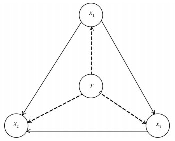
By including the time effect, the functional causal model (1) can be extended to a time-dependent functional causal model, which explains time-varying causal influences among the observed variables. As shown in Fig. 1.
|
Fig.1 Time-varying causal's graph |
The temporal information is counted as a corporate reason to other observational variables. Dotted lines express the effects of time T to the observed variables. What one mostly interested in is the causal structure among x1, x2 and x3 which is represented by solid lines.
Assume that x(t) is a multidimensional time sequences, x(t)=(x1(t), x2(t), …, xN(t))T with a limited dimension N. In light of the work[16] and to capture time-varying causal relations, we propose that x(t) obeys the following data generating models:
| $ \begin{aligned} x_{i}(t) &=\sum\limits_{j=1}^{N} \sum\limits_{p=1}^{P} a_{i, j, p}(t) x_{j}(t-p)+\\ & \sum\limits_{k \neq i} b_{i, k}(t) x_{k}(t)+s_{i}(t) \end{aligned} $ | (2) |
where si(t), i=1, 2, …, N are non-Gaussian variable that mutually independent and also independent of the reasons xj(t-p), xk(t) and t.ai, j, p(t) and bi, k(t) represent the time-varying lagged causal coefficients and the instantaneous causal coefficients respectively, and they are assumed to change over time smoothly and slowly. Note that different from the existed Gaussian noise in other model, si(t), i=1, 2, …, N in Eq. (2) are non-Gaussian variables and not limited to specific distributions.
3 Model EstimationThe part of model estimation includes the determination of causality and the estimation of the model's coefficients. Although our model belongs to causal graph model in essence, it is still a regression model. The causal graph model can infer not only from cause to result, but also from result to cause. In this paper, according to the model definition, the causality diagram which only infers from cause to result is considered, and then the granger causality test is used to ascertain the causality.
3.1 Determination of CausalityIn so far as the time sequences, the causality of granger between two variables X and Y defines as follows. In the condition of the bygone information of X and Y are known, the forecast of Y is superior to that only depends on the past information of Y. In other words, variable X is conducive to interpret prospective variation of variable Y. Then variable X is considered to be the granger causal of Y.
The time sequences must be steady is a precondition of the granger causality test. So it is necessary to deal with the time series' stationarity first by unit root test. A common method of unit root test is the augmented Dickey-Fuller test. If the sequences have a roots of unity, then it is not a stationary sequences. The granger causality test can be proceeded after proving that the time series is stationary process. Both the unit root test and the granger causality test can be done through the program named Eviews7.
The specific theory of the granger causality test is as follows, as for two stationary series {xt} and {yt} satisfy the regression model:
| $ {y_t} = c + \sum\limits_{i = 1}^n {{\alpha _i}} \cdot {y_{t - i}} + \sum\limits_{i = 1}^n {{\beta _i}} \cdot {x_{t - i}} $ | (3) |
where c is the constant term, and n is the time lagged term. Testing the variation of x is not the reason of y is equivalent to the F test of the statistical null hypothesis
| $ H_{0} : \beta_{1}=\beta_{2}=\cdots=\beta_{n}=0 $ |
The statistical test value is:
| $ F=\frac{\left(\mathrm{RSS}_{0}-\mathrm{RSS}_{1}\right) / n}{\mathrm{RSS}_{1} /(N-2 n-1)} $ |
where RSS1 is the summation of squared regression errors of formula (3), RSS0 is the summation of squared regression errors of formula (3) under null hypothesis, N is the sample size. Statistics F follow standard F distribution. Once the F inspection value is larger than the threshold of standard F distribution, then refuse the original hypothesis, and signifies that x's variation is the cause of y's. Or accept the original hypothesis and signifies that the variation of x is not the reason of y[19].
3.2 Determination of Model' s CoefficientsIn this part, a two stage approach based on ICA is proposed to estimate the coefficients of TVLC model (2). The TVLC model (2) written in matrix form as below.
| $ (\boldsymbol{I}-\boldsymbol{B}(t)) \boldsymbol{x}(t)=\sum\limits_{p=1}^{P} \boldsymbol{A}_{p}(t) \boldsymbol{x}(t-p)+\boldsymbol{s}(t) $ | (4a) |
or
| $ \begin{aligned} \boldsymbol{x}(t) &=\sum\limits_{p=1}^{P}(\boldsymbol{I}-\boldsymbol{B}(t))^{-1} \boldsymbol{A}_{p}(t) \boldsymbol{x}(t-p)+\\ &(\boldsymbol{I}-\boldsymbol{B}(t))^{-1} \boldsymbol{s}(t) \end{aligned} $ | (4b) |
where x(t)=(x1(t), x2(t), …, xN(t))T, I is the N×N identity matrix, B(t) with elements bi, k(t) is a matrix, which implies the instantaneous causal relation and could be arranged to be a strict lower triangular, Ap(t) with elements ai, j, p(t) is a matrix, s(t) with elements si(t) is a vector.
Denote
| $ \begin{array}{c}{\boldsymbol{C}_{p}(t)=(\boldsymbol{I}-\boldsymbol{B}(t))^{-1} \boldsymbol{A}_{p}(t)} \\ {\boldsymbol{z}(t)=\sum\limits_{p=1}^{P}(\boldsymbol{I}-\boldsymbol{B}(t))^{-1} \boldsymbol{A}_{p}(t) \boldsymbol{x}(t-p)} \\ {\boldsymbol{n}(t)=(\boldsymbol{I}-\boldsymbol{B}(t))^{-1} \boldsymbol{s}(t)}\end{array} $ |
then, Eq.(4) turns into:
| $ \boldsymbol{z}(t)=\sum\limits_{p=1}^{P} \boldsymbol{C}_{p}(t) \boldsymbol{x}(t-p) $ | (5a) |
| $ \boldsymbol{n}(t)=\boldsymbol{x}(t)-\boldsymbol{z}(t) $ | (5b) |
Then the estimation of the causal coefficients Ap(t), B(t) and sources s(t) in model (4) can be estimated in two steps according to Eq.(5). Cp(t) can be estimated through the Eq.(5a), and B(t) can be estimated by combine the Eq.(5b) and n(t)=(I-B(t))-1 s(t). In summary, the estimations of Ap(t) and B(t) are obtained. In the following, we describe two parts in detail.
Step 1 Estimate mixture coefficients Cp(t) of the lagged coefficients and the instantaneous coefficients.
It is easy to see that Eq. (5a) is a convolution model. Thus the problem of the model's coefficients estimation convert to a deconvolution problem. In order to solve the problem, find an inverse filter w(t) is necessary, and then recover the input data x(t)) from the output data z(t). A deconvolution algorithm based on minimum entropy[20] is applied to estimate each column of the model's coefficients Cp(t).
The algorithm is described as follows.
(1) To initialize w(0)=1, i=1.
(2) To compute iteratively x(t)) = w(t)(i-1)*z(t).
(3) To compute
(4) To compute w(i) = C-1b(i), where C is the autocorrelation matrix of series z(t).
(5) If || w(i) - w(i-1)||22 < ε, then stop iteration.
Else, let i=i+1 and then go back to (2).
When time delay p=1, the model can be denoted as z(t) = A(t)x(t)-1). As for each component of z(t),
The estimation of the mixture coefficients Cp(t) are obtained. Due to the mixture of the lagged coefficients and the instantaneous coefficients, the instantaneous coefficients are estimated next and the estimation of the lagged coefficients are obtained finally.
Step 2 Estimate the instantaneous coefficients B(t) from the noise terms.
In Eq. (4), let:
| $ \boldsymbol{n}(t)=(\boldsymbol{I}-\boldsymbol{B}(t))^{-1} \boldsymbol{s}(t) $ | (6) |
where n(t)=(n1(t), n2(t), …, nN(t))T. Because of the assumption in models that ∀t, si(t), i=1, 2, …, N are mutually independent, and ∀i, si(t) is i.i.d. noise term. Thus (Ι-B(t))-1 can be seen as a mixture matrix and Eq.(6) can be considered as a time-varying mixture ICA model. The observed variable n(t) is known, which is computed as x(t)) in Eq. (4) minus its estimation z(t) in Eq. (5), we need to estimate mixture matrix (I-B(t))-1 and s(t). For convenience, denoted (I-B(t))-1 by A(t), then the unknown variables can be estimated by the following method[21].
Suppose the general mixing process is
| $ \boldsymbol{x}(t)=\boldsymbol{A}(t) \boldsymbol{s}(t) $ |
where the component of s(t) are N independent random variables. In the case that A is an unknown N×N time independent matrix, this is also called blind signal segregation. Performing blind signal segregation means to seek the matrix J so as to y(t) = Jx(t)) gives a reconstruction of si(t). Let
| $ \begin{array}{c}{\boldsymbol{C}_{0}=E\left\{\boldsymbol{x} \boldsymbol{x}^{\mathrm{T}}\right\}= \boldsymbol{AK}(0) \boldsymbol{A}^{\mathrm{T}}} \\ {\boldsymbol{C}(\tau)=E\left\{\boldsymbol{x}(t) \boldsymbol{x}(t-\tau)^{\mathrm{T}}\right\}= \boldsymbol{AK}(\tau) \boldsymbol{A}^{\mathrm{T}}}\end{array} $ |
are the two-point correlation matrix at equal times and 2nd order cumulative matrix at time lag τ respectively. A possible practical method for obtaining J is to primarily fulfill a principal component analysis on C0 and compute the whitening matrix V, and then to find the orthogonal matrix E which diagonalizes Cz(τ)=E{z(t)z (t-τ)T}, where z(t) = Vx(t)) is the whitened mixture, then A=VE and K(τ) are estimated.
Regarding to A(t) is time-varying matrix, which is varying smoothly and relatively slowly, i.e., in any time period with scale T, there being a time size T so as to the hybrid matrix is nearly constant, i.e., the norm of dA/dt is small compared to 1/T. There-in-after, a quantity A's average means an average on the time interval [t-T, t], and can be computed as:
| $ E\{\boldsymbol{A}(t)\}=\int_{0}^{T} \frac{\mathrm{d} t^{\prime}}{T} \boldsymbol{A}\left(t-t^{\prime}\right) $ |
Hence, we get:
| $ \begin{aligned} \boldsymbol{C}_{0}=& E\left\{\boldsymbol{x}(t) \boldsymbol{x}(t)^{\mathrm{T}}\right\}=\\ & E\left\{\boldsymbol{A}(t) \boldsymbol{s}(t) \boldsymbol{s}^{\mathrm{T}}(t) \boldsymbol{A}^{\mathrm{T}}(t)\right\}=\\ & \int_{0}^{T} \frac{\mathrm{d} t^{\prime}}{T} \boldsymbol{A}(t-t^{\prime}) \boldsymbol{s}(t-t^{\prime}) \boldsymbol{s}^{\mathrm{T}}(t-t^{\prime})\cdot \\ & \boldsymbol{A}^{\mathrm{T}}(t-t) \end{aligned} $ | (7) |
| $ \begin{aligned} \boldsymbol{C}(\tau) &=E\left\{\boldsymbol{x}(t) \boldsymbol{x}(t-\tau)^{\mathrm{T}}\right\}=\\ & E\left\{\boldsymbol{A}(t) \boldsymbol{s}(t) \boldsymbol{s}^{\mathrm{T}}(t-\tau) \boldsymbol{A}^{\mathrm{T}}(t-\tau)\right\}=\\ & \int_{0}^{T} \frac{\mathrm{d} t^{\prime}}{T} \boldsymbol{A}(t-t^{\prime}) \boldsymbol{s}\left(t-t^{\prime}\right) \boldsymbol{s}^{\mathrm{T}}(t-\tau-t^{\prime})\cdot \\ & \boldsymbol{A}^{\mathrm{T}}(t-\tau-t^{\prime}) \end{aligned} $ | (8) |
On condition that the time correlation of A is feeble, we use an estimation: for every time period [t-T, t], one computes a matrix Jt such that Jt achieves signal segregation in mean on that time period.
For the sake of obtaining a well estimation of the hybrid matrix for a prescribed time interval [t-T, t], we estimate A(t-t') with a linear expansion in t' for t' from 0 to T. Then we will compute two matrices instead of computing one matrix J. The assumption on the slowly change of the hybrid matrix signifies, at 1st order, A(t-t') written as below for t' in 0 and T
| $ \boldsymbol{A}\left(t-t^{\prime}\right)=\boldsymbol{A}_{t}^{0}-\frac{t^{\prime}}{T} \boldsymbol{A}_{t}^{1} $ | (9) |
where At0 and
| $ \begin{array}{l}{E\left\{\boldsymbol{x}(t) \boldsymbol{x}(t-\tau)^{\mathrm{T}}\right\}=} \\ {\quad \int_{0}^{T} \frac{\mathrm{d} t^{\prime}}{T} \boldsymbol{A}_{t}^{0}(t-t^{\prime}) \boldsymbol{s}^{\mathrm{T}}\left(t-\tau-t^{\prime}\right) \boldsymbol{A}_{t}^{0 \mathrm{T}}-} \\ {\quad \frac{t^{\prime}}{T} \boldsymbol{A}_{t}^{1} \boldsymbol{s}\left(t-t^{\prime}\right) \boldsymbol{s}^{\mathrm{T}}\left(t-\tau-t^{\prime}\right) \boldsymbol{A}_{t}^{0 \mathrm{T}}-} \\ \quad{\frac{t^{\prime}}{T} \boldsymbol{A}_{t}^{0} \boldsymbol{s}\left(t-t^{\prime}\right) \boldsymbol{s}^{\mathrm{T}}\left(t-\tau-t^{\prime}\right) \boldsymbol{A}_{t}^{1 \mathrm{T}}-} \\ \quad{\frac{\tau}{T} \boldsymbol{A}_{t}^{0} \boldsymbol{s}(t-t^{\prime}) \boldsymbol{s}^{\mathrm{T}}\left(t-\tau-t^{\prime}\right) \boldsymbol{A}_{t}^{1 \mathrm{T}}}\end{array} $ | (10) |
And get
| $ \begin{array}{c}{\boldsymbol{C}(\tau)=\boldsymbol{A}_{\boldsymbol{t}}^{0} \boldsymbol{K}^{(0)}(\tau) \boldsymbol{A}_{t}^{0 \mathrm{T}}-\boldsymbol{A}_{t}^{1} \boldsymbol{K}^{(1)}(\tau) \boldsymbol{A}_{t}^{0 \mathrm{T}}-} \\ {\boldsymbol{A}_{t}^{0} \boldsymbol{K}^{(1)}(\tau) \boldsymbol{A}_{t}^{1 \mathrm{T}}-\frac{\tau}{T} \boldsymbol{A}_{t}^{0} \boldsymbol{K}^{(0)}(\tau) \boldsymbol{A}_{t}^{1 \mathrm{T}}}\end{array} $ | (11) |
where
| $ \boldsymbol{K}^{(k)}(\tau)=\int_{0}^{\mathrm{T}} \frac{\mathrm{d} t^{\prime}}{T}\left(\frac{t^{\prime}}{T}\right)^{k} \boldsymbol{s}\left(t-t^{\prime}\right) \boldsymbol{s}^{\mathrm{T}}\left(t-\tau-t^{\prime}\right) $ |
Note K(0)(τ) = K(τ), C(0)=C0.We can see that C(τ) is dissymmetric for nonzero τ from Eq.(11). From the aforementioned equation, it shows in the process of estimating C0 and C(τ)), a new unknown variable K(τ) is involved. To address this issue, we presume that under the integrals, the source terms can be replaced by their average,
| $ \boldsymbol{K}^{(k)}(\tau)=\int_{0}^{\mathrm{T}} \frac{\mathrm{d} t^{\prime}}{T}\left(\frac{t^{\prime}}{T}\right)^{k} \boldsymbol{K}^{(0)}(\tau)=\frac{1}{k+1} \boldsymbol{K}^{(0)}(\tau) $ | (12) |
Therefore, the correlation at time delay τ is only associated with K(0)(τ). Furthermore, a given τ only appears in the following three matrices,
| $ \boldsymbol{C}^{(1)}(\tau)=\int_{0}^{\mathrm{T}} \frac{\mathrm{d} t^{\prime}}{T} \frac{t^{\prime}}{T} \boldsymbol{x}\left(t-t^{\prime}\right) \boldsymbol{x}^{\mathrm{T}}\left(t-\tau-t^{\prime}\right) $ | (13) |
the cumulants. We obtain the below equations:
| $ 4 \boldsymbol{C}_{0}-6 \boldsymbol{C}_{0}^{(1)}=\boldsymbol{A}_{t}^{0} \boldsymbol{K}^{0} \boldsymbol{A}_{t}^{0 \mathrm{T}} $ | (14) |
| $ \begin{array}{c}{\left(4+\frac{3 \tau}{T}\right) \boldsymbol{C}^{+}(\tau)-6\left(1+\frac{\tau}{T}\right) \boldsymbol{C}^{(1)+}(\tau)=} \\ {\boldsymbol{A}_{t}^{0} \boldsymbol{K}^{(0)}(\tau) \boldsymbol{A}_{t}^{0 \mathrm{T}}}\end{array} $ | (15) |
| $ \begin{array}{c}{\boldsymbol{C}^{+}(\tau)+\frac{3 \tau}{T}\left\{\boldsymbol{C}^{+}(\tau)-2 \boldsymbol{C}^{(1)+}(\tau)\right\}=} \\ {\frac{\tau}{T} \boldsymbol{A}_{t}^{1} \boldsymbol{K}^{(0)}(\tau) \boldsymbol{A}_{t}^{0 \mathrm{T}}}\end{array} $ | (16) |
The matrices At0 and K(0)(τ) can obtain from Eqs. (14) and (15) using the same technique used to get the matrices A and K(τ) for a time independent mixture. Next, At1 can be easily computed from Eq. (16). Finally, we get the estimation of the mixture matrix A(t) according to its expansion within [t-T, t]. Meanwhile, the matrix (I-B(t))-1 can be computed and the estimation of the instantaneous coefficients can be obtained. The lagged coefficients are estimated easily using the estimated result in the first step.
After above two steps, all causal coefficients include the lagged causal coefficients and the instantaneous causal coefficients of original model are obtained. At the same time, the causality between variables are also determined. That is to say, the model estimation is finished. The effectiveness of the proposed method will be illustrated in simulation section.
4 Simulations1) Simulation 1. 2000 data are generated from the below equation which contains the time delayed and contemporary causal effect, and possesses slickly and slowly varying coefficients:
| $ \left\{\begin{array}{l}{x_{1}(t)=a_{1, 1, 1}(t) x_{1}(t-1)+a_{1, 2, 1}(t) x_{2}(t-1)+s_{1}(t)} \\ {x_{2}(t)=a_{2, 1, 1}(t) x_{1}(t-1)+a_{2, 2, 1}(t) x_{2}(t-1)+} \\ ~~~~~~{b_{2, 1}(t) x_{1}(t)+s_{2}(t)}\end{array}\right. $ |
where the coefficients possess following forms:
| $ \begin{array}{c} a_{1, 1, 1}(t)= 0.3 \cdot(\sin (t)+1.1) \\ a_{1, 2, 1}(t)=0.2 \cdot \cos (t)+0.05 \\ a_{2, 1, 1}(t)=0.2 \cdot \sin (t)+0.1 \\ a_{2, 2, 1}(t)=0.5 \cdot(\cos (t)+0.05) \\ b_{2, 1}(t)=0.2 \cdot \cos (t), s_{i}(t) \sim U[0, 1], i=1, 2 \end{array} $ |
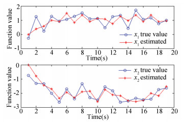
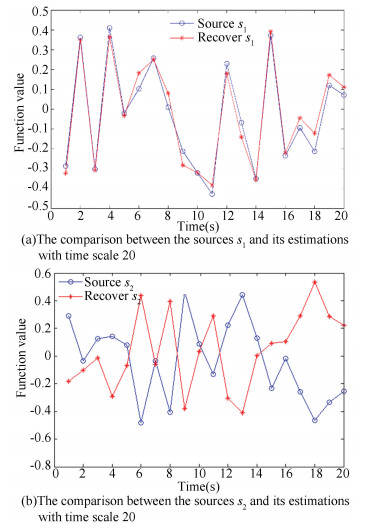
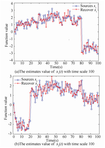
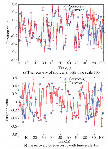
The proposed TVLC model is used to match the data and we first obtain the estimation of the mixture of the lagged coefficients ai, j, 1(t), i, j=1, 2 and the instantaneous coefficients b2, 1(t). Then we estimate the instantaneous coefficients b2, 1(t) through the mixture of noise terms and recover the sources through the proposed ICA based method. Finally, the estimation of the lagged coefficients are obtained. According to the estimated coefficients, we compare the true value and predicted value of xi(t), Fig. 2 shows the comparison between them with time scale 20. The comparison between the sources and its estimations with time scale 20 are shown in Fig. 3. It is well known that there are two indeterminacies in ICA. The indeterminacy of signs appears in the second figure in Fig. 3. We also show the estimates value of xi(t) with time scale 100 in Fig. 4 and the recovery of sources with time scale 100 in Fig. 5. For more time scale, the figure is too difficult to show the estimated effectiveness. Thus they are not shown out. From figures, the proposed method is obviously effective. Whether the comparison between the true value and predicted value of xi(t) or the comparison between the sources si(t) and its estimation, the result has a little bit of errors generated in the progress of the matrix computing. However, the overall trend are well.
|
Fig.2 The comparison between the true value and predicted value of xi(t) with time scale 20 |
|
Fig.3 The comparison between the sources and its estimations with time scale 20 |
|
Fig.4 Estimates value of xi(t) with time scale 100 |
|
Fig.5 The recovery of sources with time scale 100 |
Finally, we use granger causality test to ascertain the causality between x1(t) and x2(t) by EViews7. For this generated model, the contemporary causality between variables x1 and x2 is known from its form. The model shows that variable x1 is the instantaneous cause to variable x2. Thus, the granger causality is used here to verify the relationship between two variables. First judging the stationary of xi(t) using unit root test. The statistical value shown in Table 1 is larger than the critical value and that means xi(t) is not a stationary series. After the first difference of the series xi(t), the statistical value is smaller than the critical value and means that the 1st difference series are stationary series (as shown in Table 2). Appling granger causality test to the final series, for the model has one delay, we get that x1 is the grange cause to x2 which agrees with our generated model. The statistical result is shown in Table 3.
| Table 1 The stationary test statistical value of xi(t) |
| Table 2 The stationary test statistical value of the first difference of xi(t) |
| Table 3 The granger causality test's result |
2) Real Data Test. The daily adjust closing rates of three stock indices are chosen from 03/16/2005 to 07/31/2014, which are US's NASDAQ, UK's FTSE, and Japan's N225. The three exponents are the main stock indices all over the world, so we have a great interest in the causal relations among them. We analyze the return series of the stock indices.
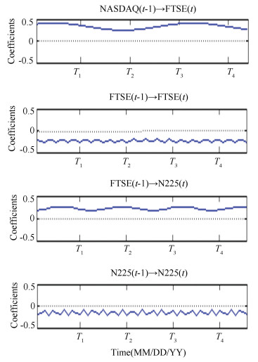
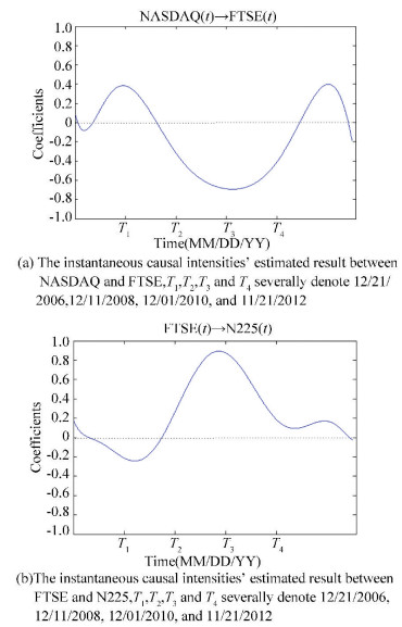
We first consider all possible pairs and test whether the granger causality test is able to find plausible causal direction. Only when the causality among three stock variables is dissymmetric can the model in Section 2 be established and the coefficients can be estimated. The granger causality test commands that the series must be stationary, so we first test the stability of the three stock indices series by the unit root test. The unit root test's results are shown in Table 4. Three series are all stationary. The granger causality test can be done to judge the right causal order between stocks. Through Eview7 the result of granger causality tests are shown in Table 5. According to the results, the test result of pair N225 and FTSER show that FTSER effect N225, pair NASDAQ and FTSER shows NASDAQ effect FTSER, and pair NASDAQ and N225 shows NASDAQ effect N225. Thus, the proposed approach favors the following causal relation NASDAQ→FTSE→N225. This really accords with the sequence on account of time lags: the time domains consistent with NASDAQ, FTSE and N225 are UTC-5, UTC, UTC+9, respectively. That is to say the granger causality test result satisfies the condition of the TVLC model. We then fit our TVLC model and estimate the various causal effects. Some of the estimated lagged causal coefficients are shown in Fig. 6 and the contemporary causal influence are shown in Fig. 7.
| Table 4 The unit root test results of three stock indices |
| Table 5 The result of granger causality tests of three stock indices |
The variation tendencies in Fig. 6 and Fig. 7 show that the causal influence of one-day delayed from FTSE to N225 is fairly little, while other lagged effects are slightly significantly. In contrast, the one-day delayed causal effects of stock itself are more significant than the causal effects from one stock to the other. The contemporary causal influences from NASDAQ to FTSE, and from FTSE to N225 are evident, which are concomitant with the effect because of the time lag. The causal coefficients become much larger from T2 to T3, this may be the result caused by the financial crisis of 2008.
|
Fig.6 Some of the lagged causal intensities' estimated result on shares, T1, T2, T3, and T4 severally denote 12/21/2006, 12/11/2008, 12/01/2010, and 11/21/2012 |
|
Fig.7 Instantaneous causal intensities' estimated result on shares |
5 Conclusions
In existing models, either the coefficients are fixed or the noise term is Gaussian, while in the proposed TVLC model, the coefficients are time-varying and the noise is non-Gaussian. In economics, neuroscience and climate analysis, the causality may alter with time and the noise is non-Gaussian, the proposed TVLC model has more widely use in practice and therefore has great research value. A two-step approach based on ICA to identify the time-varying causal influences is proposed by reserving the temporal information as a corporate reason. Under the appropriate assumptions, the method has a well estimated result. This work links the ICA based method with causality discovery and can be further studied.
| [1] |
Spirtes P, Glymour C, Scheines R. Causation, Prediction, and Search. Cambridge: The MIT Press, 2000: 50-70. DOI:10.1007/978-1-4612-2748-9
(  0) 0) |
| [2] |
Pearl J. Causality: Models, Reasoning and Inference. Cambridge: The MIT Press, 2000: 41-50. DOI:10.1017/CBO9780511803161
(  0) 0) |
| [3] |
Granger C. Testing for Causality: A Personal Viewpoint. Cambridge: Harvard University Press, 1980: 329-352.
(  0) 0) |
| [4] |
Zhang K, Hyvinen A. Causality discovery with additive disturbances: an information-theoretical perspective. Proceedings of European Conference on Machine Learning and Principles and Practice of Knowledge Discovery in Databases (ECML PKDD). Bled, 2009.570-585. DOI: 10.1007/978-3-642-04174-7_37.
(  0) 0) |
| [5] |
Shimizu S, Hoyer P O, Hyvarinen A, et al. A linear non-gaussian acyclic model for causal discovery. Journal of Machine Learning Research, 2006, 7(4): 2003-2030. (  0) 0) |
| [6] |
Hoyer P O, Janzing D, Mooij J, et al.Nonlinear causal discovery with additive noise models. In Advances in Neural Information Processing Systems, 2009 (21): 689-696.
(  0) 0) |
| [7] |
Peters J, Janzing D, Mooij J M, et al. Identifiability of causal graphs using functional models. In Proceeding of the 27th Conference on Uncertainty in Artificial Intelligence. Vancouver : AUAI Press. 2011. 589-598.
(  0) 0) |
| [8] |
Zhang K, Hyvärinen A. Causality discovery with additive disturbances: An information-theoretical perspective. Joint European Conference on Machine Learning & Knowledge Discovery in Databases. 2009. 570-585. DOI: 10.1007/978-3-642-04174-7_37.
(  0) 0) |
| [9] |
Zhang K, Hyvarinen A. On the identifiability of the post-nonlinear causal model. Conference on Uncertainty in Artificial Intelligence. Vancouver: AUAI Press. 2009. 647-655.
(  0) 0) |
| [10] |
Shimizu S, Kano Y. Use of non-normality in structural equation modeling: Application to direction of causation. Journal of Statistical Planning & Inference, 2008, 138(11): 3483-3491. DOI:10.1016/j.jspi.2006.01.017 (  0) 0) |
| [11] |
Jiang Feng, Zhu Huisheng, Wang Wei. Estimation algorithm for non-Gaussian acyclic causal model with latent variables. Computer Engineering, 2010, 36(9): 178-180. DOI:10.3969/j.issn.1000-3428.2010.09.062 (  0) 0) |
| [12] |
Hyvarinen A, Zhang K, Shimizu S, et al. Estimation of a structural vector autoregression model using non-Gaussianity. Journal of Machine Learning Research, 2010, 11(2010): 1709-1731. (  0) 0) |
| [13] |
Shimizu S. LiNGAM: Non-Gaussian methods for Estimating Causal Structures. Behaviormetrika, 2014, 41(1): 65-98. DOI:10.2333/bhmk.41.65 (  0) 0) |
| [14] |
Shimizu S, Hyvarinen A, Kano Y, et al. Discovery of non-Gaussian linear causal models using ICA. In Proc. the 21st Conference on Uncertainty in Artificial Intelligence. Vancouver: AUAI Press, 2005. 526-533.
(  0) 0) |
| [15] |
Lacerda G, Spirtes P, Hoyer P O. Discovering cyclic causal models by independent components analysis. Twenty-Fourth Conference on Uncertainty in Artificial Intelligence. Vancouver: AUAI Press, 2008. 366-374.
(  0) 0) |
| [16] |
Huang B, Zhang K, Scholkopf B. Identification of time-dependent causal model: A Gaussian process treatment. Proceedings of the 24th International Joint Conference on Artificial Intelligence. California: AAAI Press, 2015. 3561-3568.
(  0) 0) |
| [17] |
Karlsson B, Hassan M, Marque C. Windowed multivariate autoregressive model improving classification of labor vs. pregnancy contractions. Engineering in Medicine & Biology Society, 2013.7444-7447. DOI: 10.1109/EMBC.2013.6611279.
(  0) 0) |
| [18] |
Barrett A B, Michael M, Marie-Aurélie B, et al. Granger causality analysis of steady-state electroencephalographic signals during propofol-induced anaesthesia. PLoS ONE. 2012, 7(1): e29072. DOI: 10.1371/journal.pone.0029072.
(  0) 0) |
| [19] |
Lu Wanqing, Shen Peixi. The implementation of granger cause and effect test in the study of economic cycle of China. Statistical Research, 2002(2): 47-50. (in Chinese) DOI:10.3969/j.issn.1002-4565.2002.02.012.(inChinese) (  0) 0) |
| [20] |
Wang Hongchao, Chen Jin, Dong Guangming. Weak fault feature extraction of rolling bearing based on minimum entropy de-convolution and sparse decomposition. Journal of Vibration and Control, 2013, 49(1): 88-94. (in Chinese) (  0) 0) |
| [21] |
Parga N, Nadal J P. Blind source separation with time-dependent mixtures. Signal Processing, 2000, 80(10): 2187-2194. DOI:10.1016/S0165-1684(00)00076-1 (  0) 0) |
 2019, Vol. 26


