Medical images 3D reconstruction is an important step in medical image processing in spite of some existing problems and challenges. While many 3D reconstruction algorithms have been proposed continuously, reconstruction time and accuracy cannot meet the needs of actual research. Therefore, it is critical to solve the problem of reconstruction time and accuracy to meet the requirements of actual medical image analysis and processing.
In recent years, Marching Cubes (MC) algorithm has been widely applied to medical images 3D reconstruction because of its simple principles and faster speed. Garland and Heckbert used iterative edge shrinkage and quadratic error metrics to simplify complex polygonal surfaces. This surface simplification algorithm can rapidly produce high quality approximations of polygonal models. It uses iterative contractions of vertex pairs to simplify models and maintains surface error approximations using quadric matrices, and it is possible to quickly generate an approximate 3D model with slightly poorer reconstruction accuracy[1]. Zhang[2] proposed a method based on interval tree hardware acceleration, which can make the algorithm achieve 4-10 times faster speedup. Ma[3] proposed a new polyhedron model simplification method based on triangle removal criteria to speed up the rendering process, but it needs to be further improved in simplifying the selection of thresholds standard. Zhou[4] proposed a Mesh Simplification Algorithm Based on Triangle Collapse, which is a representative algorithm for improving the reconstruction speed. The mesh simplification algorithm cannot only reduce the number of triangles in the model but also maintain the model topology. Within a certain error range, by folding of the triangles in the original mesh, the processes are simplified. Moreover, Turk[5] gave a simplified method based on the re-divided polygon mesh model to achieve high frame rate in an interactive graphics application. The process of reconstructing specific details takes a long time and can generally be used for modeling but not for practical operation. Lopes and Brodlie[6] proposed a method to improve the traditional MC algorithm by triangulating and systemizing the voxel inner polygon. This method improves the robustness and accuracy of the algorithm. Lange C[7] used the denoising algorithm to improve the accuracy of 3D reconstruction. Although a lot of 3D reconstruction algorithms have been proposed or are being studied, there have always been contradictions between the speed and accuracy of the reconstruction results in the algorithms mentioned above. Therefore, it is necessary to develop a method that balances speed and accuracy.
In this paper, we propose a parallel accelerated method based on Improved Marching Cubes algorithm (I-MC) for 3D reconstruction. There are two main purposes in our study: one is to ensure the reconstruction effect of vertebrae CT images, and the other is to improve image processing speed to meet real-time requirement.
2 Bilateral Filter Point Clouds DenoisingImage preprocessing can make the results of 3D reconstruction better and more accurate. In many image processing algorithms, filtering is a key step. Vertebrae CT images contain not only needed vertebral information but also unrelated factors such as muscles, tissues and nerves, so the preprocessing of images before 3D reconstruction can eliminate irrelevant regions in medical research and enhance interest areas at the same time, which is crucial to the results of 3D reconstruction[8].
Vertebrae CT images are affected by the shape and surface state factors of the spine during scanning with the equipment. Therefore, the vertebrae CT images data should be denoised before 3D reconstruction operation. The method proposed in this paper is the bilateral filter denoising algorithm based on feature extraction. This algorithm is suitable for bone data sets. After meshing the point clouds, if they are sparse and far from the interest area, or concentrated and farther away from the center of the vertebrae, these noise point clouds are eliminated by judging the number of point clouds in each grid. However, if the noise points mix with the area of vertebrae, it is necessary to calculate the bilateral filter factors of the feature points and the non-feature point clouds respectively, then the bilateral filter point clouds denoising algorithm is used to eliminate the noise while ensuring the characteristic information of the vertebrae data sets.
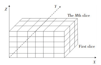
2.1 Scattered Point Clouds GridThe vertebrae point clouds data are meshed into three parts X, Y and Z according to the directions of x, y and z. In this paper, the vertebrae data sets have the resolution of 512×512. The volume data was input firstly, and 2D images were used to construct a 3D data field, then the three-dimensional coordinates were converted into one-dimensional array. At the same time, the maximum and minimum values of each coordinate could be obtained, and a cuboid data set parallel to the x, y and z axes was constructed. According to the degree of density of the data points, the cuboid data set were divided into many small cubes grids as shown in Fig. 1.
|
Fig.1 The model of three-dimensional data field |
If the minimum coordinates of the volume data sets are xmin ymin zmin, the maximum coordinates are xmax ymax zmax, and the length of the cube grid is l, then the quantity of the small cube grid in three directions are defined as follows in Eq.(1), where int represents an integer (the same as Eq.(2)), e is a natural constant, e≈ 2.718 28 (the same as Eqs.(4) and (5)).
| $ \left\{ {\begin{array}{*{20}{l}} {X = {\mathop{\rm int}} \left\{ {\frac{1}{l}\left[ {\left( {{x_{\max }} + e} \right) - \left( {{x_{\min }} - e} \right)} \right]} \right\} + 1}\\ {Y = {\mathop{\rm int}} \left\{ {\frac{1}{l}\left[ {\left( {{y_{\max }} + e} \right) - \left( {{y_{\min }} - e} \right)} \right]} \right\} + 1}\\ {Z = {\mathop{\rm int}} \left\{ {\frac{1}{l}\left[ {\left( {{z_{\max }} + e} \right) - \left( {{z_{\min }} - e} \right)} \right]} \right\} + 1} \end{array}} \right. $ | (1) |
If the coordinates of a certain point P in the data field are Px Py Pz, then the hash function of the small cube grid for this point is defined as follows in Eq.(2):
| $ \left\{ {\begin{array}{*{20}{l}} {A = {\mathop{\rm int}} \left[ {\frac{1}{l}\left( {{P_x} - {x_{\min }}} \right)} \right]}\\ {B = {\mathop{\rm int}} \left[ {\frac{1}{l}\left( {{P_y} - {y_{\min }}} \right)} \right]}\\ {C = {\mathop{\rm int}} \left[ {\frac{1}{l}\left( {{P_z} - {z_{\min }}} \right)} \right]} \end{array}} \right. $ | (2) |
where A, B, C is the index number of the grid in the three directions of the x, y and z axis. The k-nearest neighbor of a point P in the grid is sorted in ascending order of distance. If the k-nearest neighbor of the candidate points in the grid has been found, and the distance is shorter than the minimum distance from the point to the six faces of the grid, the searching of k-nearest neighbor points is finished. Otherwise, the grid expands outward and continues to search according to this rule.
2.2 Remove Noise PointsThe number of point clouds in each grid should be firstly determined. If the number is less than 2, delete all the data points directly in the grid. The purpose is to clear the scattered and sparse noise point around the volume data sets. If the number of point clouds in the grid exceeds the threshold, this grid is taken as the center, then all the surrounding grids are judged if they have data points or not. If there are data points in a grid, it is used as the center. After all the grids are viewed in turn, the adjacent grids that belong to the same point cloud are filtered out. By judging the number of grids that contain data points in each point cloud, the point cloud that contains the largest number of data point rasters can be determined. When the number of rasters in the area is not the largest, they need to be deleted so that the denser point clouds far from the research object can be removed [9].
Bilateral filter point clouds denoising algorithms was used to remove the noise points mixed with the vertebrae, p′=p-αn, where p is the original point clouds, p′ is the denoised point clouds, n is the normal direction, and β is the bilateral factor:
| $ \beta = \frac{{\sum\limits_{j = 1}^N {{W_c}} \left( {\left\| {p - {p_j}} \right\|} \right){W_s}\left( {\left\| {\left\langle {p - {p_j}, n} \right\rangle } \right\|} \right)\left\langle {p - {p_j}, n} \right\rangle }}{{\sum\limits_{j = 1}^N {{W_c}} \left( {\left\| {p - {p_j}} \right\|} \right){W_s}\left( {\left\| {\left\langle {p - {p_j}, n} \right\rangle } \right\|} \right)}} $ | (3) |
| $ {W_c}(x) = {{\rm{e}}^{ - {x^2}/\left( {2\sigma _c^2} \right)}} $ | (4) |
| $ {W_s}(x) = {{\rm{e}}^{ - {x^2}/\left( {2\sigma _s^2} \right)}} $ | (5) |
where Wc(x) is a smooth filter weight function, Ws(x) is a feature weight function, and σc, σs is a Gaussian filter coefficient on a tangent plane, σc is the length of the point nearest neighbor radius, and σs is the standard deviation of the nearest neighbor points. 〈p-pj, n〉 are two random vectors p-pj and n. ‖〈p-pj, n〉‖ is the projection of the distance vector from the data point p to the neighboring point pj.x is the abscissa of this point p.
The average Euclidean distance s of the grid point cloud and the average Euclidean distance
In order to improve the efficiency of the algorithm, we propose a method about feature extraction and triangulation configuration. GPU is used to accelerate and VTK to display the reconstructed results, then it will implement interactions, such as scaling, translation, and rotation[11-12].
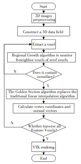
In medical image surface rendering, the class vtkMarchingCubes is provided. The general steps include: reading images, setting isosurface values, mapping, rendering, and display. The main advantages of surface rendering are rapidity and lifelikeness. The principle is constructing an intermediate geometric element with the volume data, and rendering the surface information of the target object by geometrical elements, then mapping is completed. In this paper, the seed voxels were selected, then the Region Growing algorithm was used to solve the problem about the overmuch voxels in traditional Marching Cubes algorithm. Only the voxels that contained the isosurface were extracted to reduce the searching time. At the same time, when calculated the intersection of isosurface and the voxels edge were calculated, the public edges were only calculated once. The efficiency of the algorithm was improved obviously.
I-MC is described as follows: Firstly, the original 2D vertebral CT images were preprocessed, which were used to construct a 3D data field. Secondly, the seed voxels were selected then the equivalent points were calculated. The specific process is shown in Fig. 2.
|
Fig.2 I-MC flowchart |
3.1 Feature Voxels Extraction
3D reconstruction of vertebra CT images was implemented with I-MC. Lorenson's method based on voxels surface reconstruction is a representative equidistant extraction method and is still widely used. The 3D images obtained through this method is clear and the speed of volume rendering is faster, especially for non-soft tissues such as bones. The main idea is traversing all voxels firstly. The edge voxels were determined, then isosurfaces were constructed within the edge voxels. Finally, the outline of the surface could be approximated with the edge voxels. The voxels (cubes) were sequentially processed, which is called Marching cubes algorithm[13].
In order to improve the efficiency of the algorithm, we propose a method based on the traditional MC algorithm. Due to the fact that only a small fraction of voxels contain isosurfaces, it is not necessary to traverse all voxels and waste time. In the area of interest, the seed voxels were selected first, and then Region Growing was used to select adjacent voxels that contained isosurfaces until all interested voxels were filtered out. When the intersection of the isosurface and the edge was calculated, since the adjacent voxels had common edges, it was not necessary to perform double calculations. The number of calculations of the public edges was reduced from 4 to 1, and the voxels that processed were also greatly reduced [14-17].
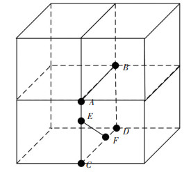
In the improved algorithm, the problem is focused on whether the voxels adjacent to the seed voxels contain isosurfaces. Each voxel contains 8 vertices and 6 faces. In Fig. 3, the four cubes are adjacent to each other, the common edge is AB, the two lower cubes (voxels) are adjacent to each other, and ABCD is the common surface, which contains four vertices A, B, C, D. If the four vertices are not greater than or less than the set threshold at the same time, adjacent voxels of the seed voxels also contain isosurfaces. In Fig. 3, the line of intersection EF is the intersection of the isosurface and the left seed voxel. Since EF exists in the right adjacent voxel, the right voxel also contains the isosurface.
|
Fig.3 Adjacent voxel isosurface and edge intersection situation |
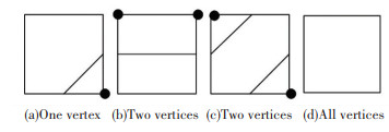
When determining whether the voxels around the seed voxels contain isosurfaces, only the state of the four vertices in the plane in that direction need to be determined. There are four situations for the states of the four vertices in the plane, as is shown in the Fig. 4: (a) has one vertex different from other states, (b) and (c) have two vertices different from other states, (d) is the same state for all vertices, so as long as four vertices are one of the three states (a), (b), and (c), then the voxels adjacent to the seed voxels have isosurfaces.
|
Fig.4 The intersection situation of isosurfaces and voxels |
3.2 Equivalent Points Calculation
After all voxels containing isosurfaces have been selected, the calculation of iso-points and normal vectors is required. In traditional algorithm, one common vertex among eight adjacent cubes needs to be calculated eight times. A common edge in four adjacent cubes is shown in Fig. 3. EF needs to be calculated four times, which seriously affects the speed of operation. In this paper, the Golden Section of the edges was used instead of the linear interpolation points, and the coordinates and normal vector of each intersection on x, y and z axes need to be calculated[18-19].
If the edge of the intersection point is on the x axis, the coordinate formula of the intersection point is:
| $ (x + (\sqrt 5 - 1)/2, y, z) $ | (6) |
If the edge of the intersection point is on the y axis, the coordinate formula of the intersection point is:
| $ (x, y + (\sqrt 5 - 1)/2, z) $ | (7) |
If the edge of the intersection point is on the z-axis, the coordinate formula of the intersection point is:
| $ (x, y, z + (\sqrt 5 - 1)/2) $ | (8) |
The normal vectors N of the intersection points on the x axis, y axis and z-axis are defined as follows:
| $ \begin{array}{l} {N_x} = N(x, y, z) + ((\sqrt 5 - 1)/2)(N(x + 1, y, z) - \\ \;\;\;\;\;\;\;\;(N(x, y, z)) \end{array} $ | (9) |
| $ \begin{array}{l} {N_y} = N(x, y, z) + ((\sqrt 5 - 1)/2)(N(x, y + 1, z) - \\ \;\;\;\;\;\;\;\;(N(x, y, z)) \end{array} $ | (10) |
| $ \begin{array}{l} {N_z} = N(x, y, z) + ((\sqrt 5 - 1)/2)(N(x, y, z + 1) - \\ \;\;\;\;\;\;\;\;(N(x, y, z)) \end{array} $ | (11) |
In this paper, the CT images of 5 lumbar, 7 cervical + 5 thoracic vertebrae, 12 thoracic + 5 lumbar vertebrae were extracted and reconstructed respectively. The data in the experiment consisted of 54, 149, and 559 CT images with the resolution of 512×512. In order to clearly compare the influence of different algorithms about the running time and accuracy, the traditional MC algorithm, Garland algorithm[1], Mesh Simplification MC algorithm[4], and the algorithm proposed by this paper respectively ran on Platform 1: Intel(R) Core(TM) i5-4590 CPU, 3.3 GHz, 8 G RAM, graphics card is AMD Radeon(TM) Windows 10, and on Platform 2: Intel ⓒ Xeon(R) CPU E5-2630 v2, 2.6 GHz x 24, 32 G RAM, GPU for NVIDIA, Quadro k4000 Ubuntu platform.
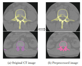
In Fig. 5, (a) is the original 2D CT image, which contains some information irrelevant to the study; (b) is the result of pre-processing by bilateral filtering de-noising algorithm, then the processed images are removed by expansion and erosion. The irrelevant part has been removed and the area of interest has been enhanced. It can be seen in Fig. 5 (b) that the contour of the interested region is clearer and the noise is effectively processed.
|
Fig.5 Original CT image and preprocessed image |
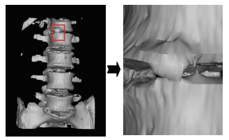
Fig. 6 shows local lumbar spine extraction and its enlargement. It can be seen that without pre-processing, the surface is not smooth and there are local loopholes in the image, and these problems will be solved in the following improved algorithm.
|
Fig.6 Reconstruction results and its partially enlarged image |
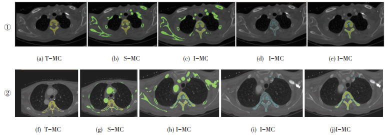
The improved algorithm proposed by this paper extracts the vertebral seed voxels and uses the region growth to obtain all the vertebral voxels in the feature extraction of the 2D CT images. The accurate extraction of vertebrae features makes the 3D images more accurate after reconstruction. Because both Mesh Simplification MC algorithm (S-MC) and Garland algorithm (G-MC) have advantages in improving the reconstruction speed, when comparing the reconstruction accuracy, we chose the Mesh Simplification MC algorithm as a representative, and compared it with the Traditional MC algorithm (T-MC) and the Improved MC algorithm (I-MC) of this paper.
Fig. 7 (a), (f) are the result of feature extraction by T-MC algorithm in 2D image, Fig. 7 (b), (g) are the effect of the S-MC algorithm after extracting feature information, Fig. 7 (c), (d), (e) and (h), (i), (j) are the processes of feature extraction in I-MC. Firstly, the interest area and the non-interest area were distinguished. Secondly, the edges were marked and extracted by using the idea of region growth. Finally, all the voxels containing the isosurface were extracted, and the vertebral area to prepare for the later 3D reconstruction was determined. It can be concluded from Fig. 7 that I-MC can accurately extract the vertebral region and mark it effectively in the feature extraction process, which is crucial for improving the accuracy of 3D reconstruction.
|
Fig.7 Comparison of 2D CT image feature extraction |
After analyzing the 2D images, the 3D reconstruction of 7 cervical vertebrae + 5 thoracic vertebrae were implemented with these three algorithms respectively. Then the reconstruction accuracy was compared by calculating the repetition rate of the characteristic voxels. This vertebral data contains 149 CT images with the resolution 512×512 and each CT image interval is 1.4 mm.
As shown in Fig. 8, (a) is the effect of T-MC algorithm for 3D reconstruction and comparison with the overall data set (including soft tissue). (b) is the effect of S-MC algorithm for 3D reconstruction and comparison with the overall data set (c) is the result of I-MC for 3D reconstruction and comparison with the overall data set (including soft tissue).

|
Fig.8 Comparison of 3D reconstruction effect |
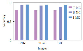
Fig. 8 shows that the 3D reconstruction result of I-MC is smoother, and the degree of fitting with the original data set is higher. The images of detailed reconstruction accuracy in Fig. 7 and Fig. 8 are shown in Table 1.
| Table 1 Comparison of reconstruction accuracy of several algorithms |
From Table 1, the comparison of the reconstruction accuracy of different algorithms is shown clearly, thus the reconstruction accuracy statistics of each algorithms are obtained as shown in Fig. 9. Regardless of feature extraction in 2D images or comparison of effects after 3D reconstruction, I-MC has some advantages. The reconstruction speed of the four algorithms was studied subsequently.
|
Fig.9 Comparison of reconstruction accuracy |
The experiment data were obtained from three different patients in a hospital in Xi'an: 5 lumbar vertebrae, containing 54 CT images, with an interval of 2.5 mm; 7 cervical vertebrae +5 thoracic vertebrae, containing 149 CT images, with an interval of 1.4 mm; 12 thoracic vertebrae +5 lumbar vertebrae, containing 559 CT images, with an interval of 1mm. The four algorithms in the experiment were reconstructed on two platforms. The reconstruction time of the four algorithms for the three data sets is shown in Table 2 and Table 3.
| Table 2 Comparison of the reconstruction speed of several algorithms on Platform 1 |
| Table 3 Comparison of the reconstruction speed of several algorithms Platform 2 |
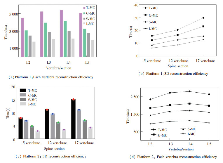
From Table 2, Table 3, and the experiment of reconstructing 5 lumbar spines respectively, the statistics of reconstruction time can obtained as shown in Fig. 10. (a), (c) are the charts showing the reconstruction time of 2-5 lumbar vertebrae on platforms 1 and 2. (b), (d) are the 5 vertebrae, 12 vertebrae and 17 vertebrae reconstruction time with four algorithms on platform 1 and 2. It can be seen that the I-MC has great advantages in running time on the two platforms.
|
Fig.10 Reconstruction efficiency of different algorithms |
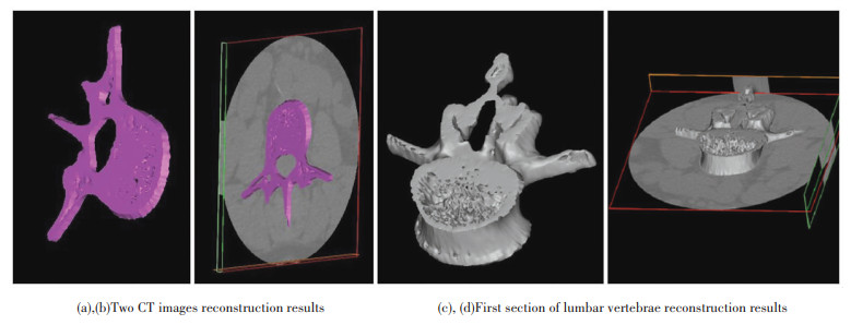
Fig. 11 shows the reconstruction results of the I-MC. Fig. 11(a), (b) are the two CT images reconstruction results. Fig. 11 (b) contains background information, which helps to easily compare the reconstruction accuracy. Fig. 11(c), (d) are the first section of lumbar vertebrae reconstruction results. Fig. 11 (d) contains background information. It can be seen from Fig.11 that the reconstruction effect of I-MC is satisfactory. The reconstructed images basically fit the original images and can meet the requirement of real-time medical diagnosis and research.
|
Fig.11 Two CT images and first section of lumbar vertebrae reconstruction |
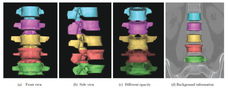
Fig. 12 shows the reconstruction results of 5 lumbar vertebrae. Fig. 12 (a) is a front view and Fig. 12 (b) is a side view. As shown in Fig. 12 (c), different opacity can be set for each section of vertebrae according to different needs, and the vertebrae in which the lesion area is located can also be made transparent, which is conducive to the observation of the internal structure of the vertebrae. Fig. 12 (d) is the reconstruction results with background information, showing that the vertebral surface is smooth and the reconstruction effect is better.
|
Fig.12 Reconstruction results of 5 lumbar vertebrae |
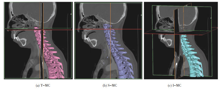
Fig. 13 shows the reconstruction results of 7 cervical vertebrae + 5 thoracic vertebrae with T-MC, S-MC and I-MC separately. Fig. 13 (a) is the T-MC algorithm, and Fig. 13 (b) is the S-MC algorithm. The reconstruction results show that the S-MC algorithm is better than the T-MC algorithm, but there are still some loopholes and flaws. Fig. 13 (c) is the reconstruction results of I-MC. Problems existing in the T-MC algorithm and the S-MC algorithm can be well solved by denoising, feature extraction, and 3D reconstruction in I-MC. It provides construction result with better smoothness, higher accuracy, and faster speed.
|
Fig.13 Reconstruction results of 7 cervical + 5 thoracic vertebrae |
Fig. 14 shows the reconstruction of 12 thoracic + 5 lumbar vertebrae. Doctors and researchers can extract any piece of vertebral data according to actual needs and research requirement. The reconstruction result generated by I-MC can simultaneously satisfy real-time and accuracy needs.

|
Fig.14 Reconstruction results of 12 thoracic + 5 lumbar vertebrae |
5 Conclusions
In this paper, the reconstruction method of Improved Marching Cubes algorithm (I-MC) is proposed, which can solve the problem of reconstruction time and accuracy that cannot be solved by the traditional MC algorithm. Compared with the traditional MC algorithm, Garland algorithm, and the Mesh Simplification MC algorithm, we improve the reconstruction speed while preserving accuracy at the same time. The number of voxels is reduced by about 400 times, and equivalent points calculation time is drastically reduced. Accuracy can be guaranteed above 95.5%. The experimental results show that the efficiency of traditional MC algorithm is significantly improved. I-MC is suitable for all vertebral CT images, but according to different vertebral image data, the reconstruction effect will be slightly different. In the process of visualization after reconstruction on VTK, different display effects are set according to different research needs, which is crucial to the success of the experiment. However, the 3D reconstruction of the vertebrae internal structure needs to be further improved. Future work will focus on the reconstruction of internal structure of vertebrae, and we will prepare for the study of the precise placement of pedicle screws.
| [1] |
Garland M, Heckbert P S. Surface simplification using quadric error metrics. Proceedings of the 24th annual conference on Computer Graphics and Interactive Techniques. New York: ACM Press/ Addison-Wesley Publishing Co., 1997: 209-216. DOI:10.1145/258734.258849
(  0) 0) |
| [2] |
Zhang Y, Gao G, Lu Y, et al. Hardware-acceleration interval tree index for marching cubes. Journal of Computer - Aided Design and Computer Graphics, 2012, 24(7): 871-878. (  0) 0) |
| [3] |
Ma Xiaohu, Pan Zhigeng, Shi Jiaoying. Delaunay triangulation of simple polygon based on determin ation of convex-concave vertices. Journal of Computer-Aided Design & Computer Graphics, 1999, 11(1): 2-4. (  0) 0) |
| [4] |
Zhou Kun, Pan Zhi-Geng, Shi Jiao-Ying. Mesh simplification algorithm based on triangle collapse. Chinese J. of Computer, 1998, 21(6): 506-513. (  0) 0) |
| [5] |
Turk M, Pentland A. Eigenfaces for Recognition. Journal of Cognitive Neuroscience, 1991, 3(1): 71-86. DOI:10.1162/jocn.1991.3.1.71 (  0) 0) |
| [6] |
Lopes A, Brodlie K. Improving the robustness and accu-racy of the marching cubes algorithm for isosurfacing. IEEE Transactions on Visualization and Computer Graphics, 2003, 9(1): 16-29. DOI:10.1109/TVCG.2003.1175094 (  0) 0) |
| [7] |
Lange C, Polthier K. Anisotropic smoothing of point sets. Computer Aided Geometric Design, 2005, 22(7): 680-692. DOI:10.1016/j.cagd.2005.06.010 (  0) 0) |
| [8] |
Yang M, Lee E. Segmentation of measured point data using a parametric quadric surface approximation. Computer-Aided Design, 1999, 31(7): 449-457. DOI:10.1016/S0010-4485(99)00042-1 (  0) 0) |
| [9] |
Cao Shuang, Yue Jianping, Ma Wen. Bilateral filtering denoise algorithm for point cloud based on feature selection. Journal of Southeast University (Natural Science Edition), 2013, 43(S2): 351-354. DOI:10.3969/j.issn.1001-0505.2013.S2.029 (  0) 0) |
| [10] |
Piegl L A, Tiller W. Algorithm for finding all k nearest neighbors. Computer-Aided Design, 2002, 34(2): 167-172. DOI:10.1016/S0010-4485(00)00141-X (  0) 0) |
| [11] |
Wen Tiexiang, Yang Feng, Gu Jia, et al. An adaptive kernel regression method for 3D ultrasound reconstruction using speckle prior and parallel GPU implementation. Neurocomputing, 2017, 275(31): 208-223. DOI:10.1016/j.neucom.2017.06.014 (  0) 0) |
| [12] |
Kitware Inc. VTK User's Guide. 11th ed. New York: Kitware Inc, 2010: 8-90.
(  0) 0) |
| [13] |
Lorensen W E, Cline H E. MarchingCubes: A high resolution 3D surface construction algorithm. ACM SIGGRAPH Computer Graphics, 1987, 21(4): 163-169. DOI:10.1145/37402.37422 (  0) 0) |
| [14] |
Dietrich C A, Scheidegger C E, Schreiner J, et al. Edge transformations for improving mesh quality of marching cubes. IEEE Transactions on Visualization and Computer Graphics, 2009, 15(1): 150-159. DOI:10.1109/TVCG.2008.60 (  0) 0) |
| [15] |
Zhu Kai, Fan Lingzhong, Li Haifang. 3D reconstruction of brain atlas based on modified marching cubes algorithm. Computer Applications and Software, 2009, 15(1): 150-159. DOI:10.3969/j.issn.1000-386x.2016.04.042 (  0) 0) |
| [16] |
Nugroho P A, Basuki D K, Sigit R. 3D heart image reconstruction and visualization with marching cubes algorithm. 2016 International Conference on Knowledge Creation and Intelligent Computing (KCIC). Piscataway: IEEE, 2017: 35-41. DOI:10.1109/KCIC.2016.7883622
(  0) 0) |
| [17] |
Liu Xia, Cao Yang, Cao Yu, et al. Novel method fusing (2D)2LDA with multichannel model for face recognition. Journal of Harbin Institute of Technology(New Series), 2015, 22(6): 110-114. DOI:10.11916/j.issn.1005-113.2015.06.015 (  0) 0) |
| [18] |
Shuai Renjun, Chen Shujing. An improved MC 3D reconstruction algorithm. Chinese Digital Medicine, 2016, 11(3): 83-86. DOI:10.3969/j.issn.1673-7571.2016.03.028 (  0) 0) |
| [19] |
Wang Xinsheng, Yu Mingyan. Weighted self-adaptive threshold wavelets for interpolation point selection used in interconnect MOR. Journal of Harbin Institute of Technology(New Series), 2018, 25(1): 39-45. DOI:10.11916/j.issn.1005-9113.16119 (  0) 0) |
 2019, Vol. 26


