2. Institute of Architecture and Civil Engineering, East China Jiaotong University, Nanchang 330013, China
In many applications, we need better information about the obtained data. Sometimes, the complexity of the data with non-stationary characteristics would lead to diverse periodic events occurred in different time periods. To detect the periods of the observed data is regarded as a meaningful thing. In order to optimize the results, it requires not only the time series have adequate length, but also requires the appropriate mathematical tools are used.
In detecting the precipitation with increasing or decreasing trend and period, wavelet method is one powerful tool. The method has been widely used in many fields in order to analyse the data set from two aspects in the same time: frequency domain and time domain. In most practical applications, discrete wavelet transform (DWT) is used to analyse the trends and periods of precipitation as discussed by Niu et al[1-8]. Partal et al.[9] studied the precipitation of 64 years in Marmara region, Turkey through using DWT analysis. Xing et al.[10] found that it is a fast and effective way to detect and compare the similarity of different hydrological series by using the DWT analysis. Lots of studies have showed that low frequency fluctuations at decadal and higher time scales could give rise to extreme floods or droughts. In the pervious research, all used wavelet transform was classicial wavelet functions, such as Haar wavelet, Daubechies wavelet, Mexican Hat wavelet, Meyer wavelet, Morlet wavelet, et al[11-13]. The programs of these classicial wavelets could be found in Matlab toolkits. When using classicial wavelet method the researcher has to decide the wavelet scale and wavelet basis firstly. While different chosen wavelet scale and wavelet basis would lead to different results. Sometimes, the difference is great. In order to overcome this shortcoming, Yu et al.[14] introduced the concept of the Natural-based wavelet method. In the present paper the new method, that is, the Natural-based wavelet method is derived detailed. More importantly, the novel method only needs the information of record data set. In addition, when new information appears, it can be easily extended to new information. This is another advantage of the proposed method. As discussed in later sections the Natural-based wavelet can be regarded as a special class of discrete wavelets which can reflect multi-time scale periods of time sequence.
Let the observed temporal series (such as temperature, precipitation, pressure etc.) be denoted by
| $ \mathit{\boldsymbol{X}} = {\left( {x\left( {{t_1}} \right), x\left( {{t_2}} \right), \cdots , x\left( {{t_n}} \right)} \right)^{\rm{T}}} $ |
where ti=t1+iΔt, i=0, 1, …, N-1. Take even time interval Δt. Suppose in sequence X, the wave whose wavelength is l(2≤l≤N/2) can be found. Let index s=N-(m-1)×l, m=[N/l].
Therefore, vector X can be reshaped by matrix
| $ \mathit{\boldsymbol{\tilde X}} = \left( {\;\begin{array}{*{20}{c}} {{{\tilde x}_{11}}}&{{{\tilde x}_{12}}}& \cdots &{{{\tilde x}_{1s}}}&{{{\tilde x}_{1(s + 1)}}}& \cdots &{{{\tilde x}_{1l}}}&{}\\ {{{\tilde x}_{21}}}&{{{\tilde x}_{22}}}& \cdots &{{{\tilde x}_{2, }}}&{{{\tilde x}_{2(s + 1)}}}& \cdots &{{{\tilde x}_{2l}}}&{}\\ \cdots & \cdots & \cdots & \cdots & \cdots & \cdots & \cdots &{}\\ {{{\tilde x}_{m1}}}&{{{\tilde x}_{m2}}}& \cdots &{{{\tilde x}_{ms}}}&0& \cdots &0&{} \end{array}} \right) $ |
where element
In the last line of matrix
| $ \begin{array}{l} \;\;\;\;\;\;\;{{\mathit{\boldsymbol{\tilde X}}}^w} = \left( {\begin{array}{*{20}{c}} {\tilde x_{11}^w}&{\tilde x_{12}^w}& \cdots &{\tilde x_{1, }^w}&{\tilde x_{1(s + 1)}^w}& \cdots &{\tilde x_{1l}^w}\\ {\tilde x_{21}^w}&{\tilde x_{22}^w}& \cdots &{\tilde x_{2s}^w}&{\tilde x_{2(s + 1)}^w}& \cdots &{\tilde x_{2l}^w}\\ \ldots & \cdots & \cdots & \cdots & \cdots & \cdots & \cdots \\ {\tilde x_{m1}^w}&{\tilde x_{m2}^w}& \cdots &{\tilde x_{ms}^w}&0& \cdots &0 \end{array}} \right)\\ {\rm{where}}\;\tilde x_{ji}^w = {{\tilde x}_{ji}} - \bar X.\\ \;\;\;\;\;\;\;{\rm{Let}}\\ \;\;\;\;\;\;\;\tilde x_i^w = \left\{ {\begin{array}{*{20}{l}} {\frac{1}{m}\sum\limits_{j = 1}^m {\tilde x_{ji}^w} , }&{1 \le i \le s}\\ {\frac{1}{{m - 1}}\sum\limits_{j = 1}^{m = 1} {\tilde x_{ji}^w} , }&{s + 1 \le i \le l} \end{array}} \right. \end{array} $ |
Two indexes S2and D2 are defined by:
| $ \begin{array}{l} {S^2} = \sum\limits_{j = 1}^m {\sum\limits_{i = 1}^s {{{\left[ {\tilde x_{ji}^w - \tilde x_i^w} \right]}^2}} } + \sum\limits_{j = 1}^{m - 1} {\sum\limits_{i = s + 1}^l {{{\left[ {\tilde x_{ji}^w - \tilde x_i^w} \right]}^2}} } \\ \;\;\;\;\;\;\;\;\;\;\;\;\;\;\;\;\;\;\;\;\;\;\;{D^2} = \sum\limits_{i = 1}^l {{{\left( {\tilde x_i^w} \right)}^2}} \end{array} $ |
By mathematical statistical theory, in a certain conditions, statistics F=[D2(n-l)]/[S2(l-1)] almost obeys to F(l-1, n-l)-distribution. If confidence level 1-α is taken relatively large (for example α=0.05) and corresponding value F≥Fα, that is time sequence (x(t1), x(t2), …, x(tl))T passes through F-test to be a basis of the Natural-based Wavelet with the wave length l. The error estimation can be referenced relevant books.
For an observed time sequence, the process of searching for the basis of Natural-based Wavelet is as follows:
1) At the beginning, the wavelength l is taken to 2 (or N/2).
2) Increasing (or decreasing) l, suppose the k-th wavelet length 2≤lk≤N/2 passed through F-test, then the k-th wavelet residual sequence is obtained by (k-1)-th wavelet residual sequence from subtracting the Natural-based wavelet. Thus, one of distinguished periods will be lΔt.
3) Repeating process 2) until l=N/2 (or l=2), all obtained Natural-based wavelet set constitutes the basis of Natural-based Wavelet Method.
2 Numerical ExamplesIn this section some examples are designed to show the capability of Natural-based Wavelet Method. The first example is:
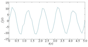
| $ {f_1}(t) = 10\sin (2{\rm{ \mathit{ π} }}t) + \varepsilon (t) $ |
where ε(t)~N(0, 1) is a white noise series on time interval [0, 5]. Time step Δt is taken to 0.1 s. In fact, for function f1(t) the exact period equals to 1 s and the exact frequency equals to 1 Hz. The figure of function f1(t) is shown in Fig. 1. By using Natural-based wavelet method, under the significance level α=0.005, l=10 is remarkable. The corresponding p-value is smaller than 10-10. So the computed period equals to 1 s. The result is exactly true.

|
Fig.1 Figure of function f1(t) |
The second example is:
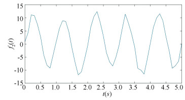
| $ {f_2}(t) = 10\sin (2{\rm{\pi }}t) + 2\sin ({\rm{\pi }}t) + \varepsilon (t) $ |
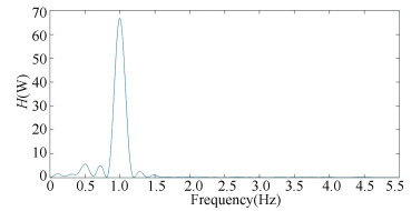
All parameters are set up as the same as the parameters in example 1. It is well known that for function f2(t), there exist two major periodic components 1 and 2 s. Thus the corresponding frequencies are 1 and 0.5 Hz. The figure is shown in Fig. 2 and the result obtained by Fourier Analysis is shown in Fig. 3. For the Natural-based Wavelet Method, under the significance level α=0.005, l=10 and 18 are both remarkably. Especially when T=10Δt, the corresponding p-value. is almost 0. When T=18Δt, p-value. is smaller than 10-5. While in Fig. 3 the frequency 0.5 Hz is not so obvious. This example has showed that in multi-frequency time sequence the proposed N-wavelet method is more accurate than fourier transform.

|
Fig.2 Figure of function f1(t) |

|
Fig.3 Figure of frequency-power of function f2(t) |
If time step is shortened to 0.05 s, the other parameters are remaining the same as the parameters in example 2. The computed periods l=19, 21, 34, 35 and 45Δt are all remarkable. Although the computed periods are near to the exact periods, but they are not the same. One of the feasible criterions is to take the period which has the smallest p-value.
From these two examples, some conclusions or criteria can be made.
1) The noise included in the data cannot be dominant.
2) Time resolution cannot be taken highly. When time resolution is fine, there may exist pseudo-periodicity. Thus one feasible criteria is to take the period which has the smallest p-value.
3) The proposed N-wavelet Method can be used in multi-resolution time sequence in order to distinguish the period. The computed results are better than the results obtained from Fourier Transform.
3 Natural-based Wavelet Analysis and PredictionIn this section the N-wavelet Method is used to analyze the trend and period in precipitation[15-17]. The length of the annual precipitation series is 110 years. Time step Δt is taken to 1 year.
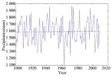
The annual precipitation is shown in Fig. 4. It can be seen the mean annual precipitation is 1 590.5 mm. The regression function is y=1 344.4t+0.125 9, where y is precipitation, and t is time. This result states that the precipitation has a faintly increasing trend. Every 100Δt the precipitation increases 12 mm.

|
Fig.4 Precipitation (red line denotes regression) |
The length of the precipitation is 110 years. First the sequence is divided into 5 different subsequences: R1-103, R2-104, R3-105, R4-106 and R5-107 year. According to the analysis discussed in previous sections possible periods existed in these annual precipitation sequences may vary from 2 to 52 years. The computed periods of these 5 sequences are rather concentrated on 41 years under the significance level α=0.05. The results are shown in Table 1.
| Table 1 Comparison between predicted and observed precipitation (Unit: mm, time interval is 104 years) |
In order to examine the ability of prediction of Natural-based wavelet method, short range forecasting (3 time steps) is made. For reducing the random of prediction, average prediction is used and average relative error (ARE) is defined by:
| $ \begin{array}{l} {E_{{\rm{ARE}}}} = ({\rm{ average }} - {\rm{ prediction\;observed }})/\\ \;\;\;\;\;\;\;\;\;\;{\rm{observed}} \times 100\% \end{array} $ |
It is clear in Table 1.
1) In these five sequences, there appeared six periods, that is, 33, 48, 11, 41, 29 and 52 years. In the first two sequences the major periods are 33 and 48 years. In the last three sequences 11 and 41 years are both remarkable. Especially, in the last two sequences 29 and 52 years are also apparent.
2) The largest relative error in following three time steps forecasting is no more than 30%. The smallest relative error is about -0.4%. Most forecasts are coincided with actual precipitation. The results are perfect. Thus the proposed method can be used in practice for some purpose.
In order to compare the results obtained by predicted and actual precipitation. The time interval is reduced to 50 years. The results are shown in Table 2.
| Table 2 Comparison between predicted and actual precipitation (Unit: mm, time interval is 50 years) |
In Table 2, it can be seen the largest relative error in three time steps forecasting is also no more than 30%. The smallest relative error in forecasting is about 0.7%. The results are similar to Table 1. Shortening the length of time interval, the precision is improved only a little. The reasons may be [18-19]:
1) In long range precipitation sequence, the observed error may be larger since of technical reasons. With technology improving, various observed errors decrease. When shortening the length of time sequence, the computed periods do not vary so much.
2) In long range precipitation sequence, there exist unusual points and inflection points.
3) The process of precipitation is an extremely complex process and many mechanisms cannot be clearly understood now. All these reasons need further studies.
4 ConclusionsIn the present paper, the basis concepts and theories about Natural-based Wavelet Method were introduced briefly. Two examples were designed to demonstrate capability of the proposed method in distinguishing periods both in single frequency time series and in multi-frequency time series. At last, the proposed method was used to an observed precipitation sequence. The obtained results validated that:
1) In multi-frequency serials, N-wavelet Method is more precise than classical Fourier Transform.
2) When using N-wavelet Method, time resolution cannot be taken so fine, one feasible criterion is to choose the smallest p-value.
3) Natural-based Wavelet Method is suitably used in complicated observed data and can be used to make short range precipitation prediction. The proposed method is novel and easy to program. When new information appears, new information can be easily added into the original sequence.
| [1] |
Niu C W, Zhang L P, Xia J. Wavelet analysis on the precipitation in North China. Arid Land Geography, 2004, 27(1): 66-70. (in Chinese) (  0) 0) |
| [2] |
Li M, Xia J, Chen S M, et al. Wavelet analysis on annual precipitation around 300 years in Beijing area. Journal of Natural Resources, 2011, 26(6): 1001-1011. (in Chinese) DOI:10.11849/zrzyxb.2011.06.011.(inChinese) (  0) 0) |
| [3] |
Hu Y N, Wang L H, Zhang G S, et al. Wavelet analysis on the temporal series of principal climate factors in Mu Us Sandy Land during 1969-2009. Journal of Desert Research, 2013, 33(2): 390-395. (in Chinese) (  0) 0) |
| [4] |
Min Q. Analysis on the flood characters in 1990's Poyang Lake. Journal of Lake Science, 2002, 14(4): 323-330. (in Chinese) (  0) 0) |
| [5] |
Zhan L S, Yuan W L, Min Q, et al. Correlation between the cycles of solar activities and the flood occurrences in the Poyang Lake. Astronomical Research & Technology, 2009, 6(3): 175-180. (in Chinese) (  0) 0) |
| [6] |
Heil C E, Walnut D F. Continuous and discrete wavelet transforms. SIAM Review, 1989, 31(4): 628-666. DOI:10.1137/1031129 (  0) 0) |
| [7] |
Kim S. Wavelet analysis of precipitation variability in Northern California. U.S.A. KSCE Journal of Civil Engineering, 2004, 8(4): 471-477. DOI:10.1007/BF02829169 (  0) 0) |
| [8] |
Li R F, Wang P, Wu D Y. Wavelet analysis of annual precipitation series in Poyang lake basin. Journal of China Hydrology, 2012, 32(1): 29-31. (in Chinese) (  0) 0) |
| [9] |
Partal T, Kahya E. Trend analysis in Turkey precipitation data. Hydrologic Processes, 2006, 20: 2011-2026. DOI:10.1002/hyp.5993 (  0) 0) |
| [10] |
Xing C, Wang H F, Yu F. Detection and comparison of hydrologic series based on discrete wavelet transform analysis. Science and Technology Information, 2010, 23: 47-48. (  0) 0) |
| [11] |
Zhao R Z, Liu X Y, Li C C, et al. Wavelet denoising via sparse representation. Science China Series F: Information Sciences, 2009, 52(8): 1371-1377. DOI:10.1007/s11432-009-0116-7 (  0) 0) |
| [12] |
Jiang Z Q, Gao X L, Zhou W X, et al. Multi-fractal cross wavelet analysis. Fractals, 2017, 25(6): 1-10. DOI:10.1142/S0218348X17500542 (  0) 0) |
| [13] |
Guo H F, Qiu X, Liu Y L. Application of wavelet analysis in numerical study of turbulence. Chinese Journal of Computational Mechanics, 2006, 23(1): 58-65. (  0) 0) |
| [14] |
Yu K Q, Zhou Y H, Yang J A, et al. Natural-base analyses and short-range climatic prediction for meteorological element time series. China Meteorological Society 2006 Annual Meeting. Beijing, 2006. 991-1005. (in Chinese)
(  0) 0) |
| [15] |
Yuan L F, Yang G S, Li H P, et al. Fainfall multiple time scale variation rule of Poyang Lake basin in the past 50 years. Resources and Environment in the Yangtze Basin, 2014, 23(3): 434-440. (  0) 0) |
| [16] |
Xu W M, Dun M. The variation of Poyang Lake hydrological regime and its cause analysis. Jiangxi hydraulic Science & Technology, 2013, 39(3): 161-163. (  0) 0) |
| [17] |
Cao Y H, Ye X F, Liu X M. Analysis of the influence of Poyang Lake on convective systems and lightning transited. Progress in Civil, Architectural and Hydraulic Engineering Ⅳ-Kim (Ed.), 2016, 639-642. (  0) 0) |
| [18] |
Cao Y H, Ye X F, Lv G H. Analysis of precipitation characteristics of Poyang Lake Basin. Applied Mechanics and Materials, 2014, 641-642: 29-32. DOI:10.4028/www.scientific.net/AMM.641-642.29 (  0) 0) |
| [19] |
Cao Y H, Lv G H, Yi H. Multi-scale analysis of long time precipitation series in Poyang Lake Basin. Journal of East China Jiaotong University, 2016, 33(3): 121-125. (  0) 0) |
 2019, Vol. 26


